

In this article, we will discuss all the core concepts of Spark API; however, our focus is to use Spark for data science. The details about the big data framework provided in the article will be sufficient for you to understand performing data science with Spark. For data collection and storage, Spark has a very nice distributed mechanism that uses RDD. For data cleaning and data processing, Spark provides a DataFrame API, which is available in Java, Python, R, and Scala. In this article, we will be using the API for Python, wherever needed.
Data Lifecycle
The data lifecycle consists of various steps involved in getting insights from data. We obtain raw data from various sources and then integrate, explore, and aggregate the data. This helps reduce the volume of data (perhaps from terabytes to gigabytes). Once the data is in an organized and structured format, we further narrow down the data as it is suitable for the use case or business problem in hand. We find patterns, trends, predictions, and build a model that can be deployed and then monitored to get the insights required.
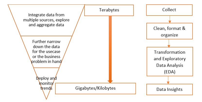
In the collection, we get data from various sources, like social media sites, databases, CSV files, and XML files. All that data has to be integrated into a single source. The data then should be formatted in a single understandable common format, like Parquet, Avro, and text.
Big Data
We have said that the data comes from various sources, which means it has to be a huge chunk of data of millions of users. You might be knowing about how Facebook receives more than 100k likes every minute or 3 hours of video is uploaded on YouTube every single minute. Imagine collecting data for a day, week, month, and so on. That will be huge! And all of it – raw! Well, the volume of data coming from a variety of sources (like Instagram and Facebook) is just one part of it. The data multiplies very fast, i.e., the velocity of the data becoming huge is very high. Even if the data is not voluminous, it is complex because of its unstructured nature. The veracity (integrity) and the value of the data are other important aspects of big data. These are called the 5 V’s of big data and constitute the definition of big data – Volume, Variety, Velocity, Veracity and Value. Because of the above complexities, RDBMS systems are not suitable for big data. Thus, we need something more flexible and reliable, like Apache Spark.
Big Data Analytics
Big data analytics is a process where large datasets are analyzed to find hidden patterns, trends, correlations, customer preferences, and other insights. There are two main aspects of big data analytics – storage and processing. Big data analytics is also of 2 types – Batch analytics and Real-time analytics. In batch analytics, data is collected and stored over a period of time, and then ETL is performed on the data. Some examples are credit card data and call data collected over some time. The MapReduce function of Hadoop can perform batch analytics on the data collected over a period of time. Real-time analytics is a type of big data analytics that is based on real-time (immediate/streaming) data for immediate results. Data from IoT devices, cloud, GPS devices are some examples of real-time analytics data. Although Hadoop is a great big data framework , it cannot take care of real-time analytics. It can only work on already stored data i.e. batch. That is why we need Apache Spark. There are a few more reasons why data science with Spark is a better option for data processing, but before discussing that let us first quickly learn what Apache Spark is.
What is Apache Spark?
Apache Spark is a cluster-computing framework with support for lazy evaluation. It is known for its speed and efficiency in handling big chunks of data. Spark is an open-source unified engine for data processing and analytics. The computations in Spark run in the memory. This is in contrast to MapReduce, where applications run on the disk.
Spark Architecture
Spark has a very simple architecture and consists of 3 main parts:
- The driver program,
- Cluster manager, and
- Worker nodes.
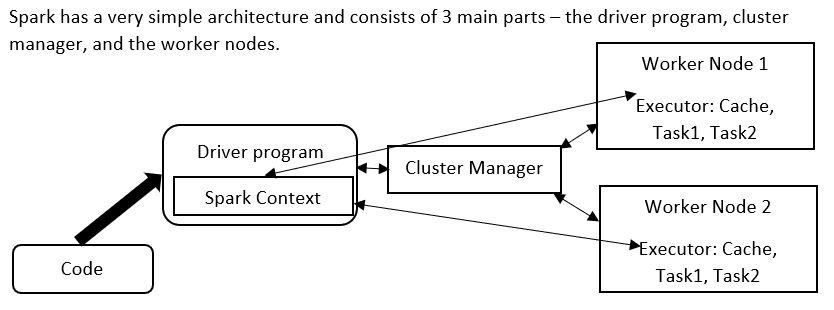
The Spark Context is like the main() function in Java or C++. It is the main entry point of a Spark application. Application code is sent to the driver program, which has the Spark Context. The Spark Context initializes the cluster manager, which splits the data into different worker nodes. The executor is similar to JVM (Virtual machine) that does memory management. The executors have tasks that share access to the cache.
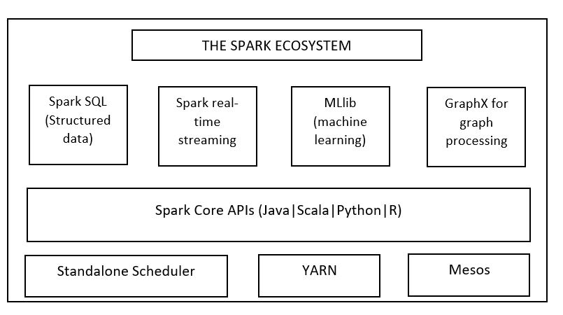
The Spark Ecosystem
Spark provides an entire framework for data processing and analysis. This is why it is called a unified engine. It has the following components:
-
Spark Core API
The Core API contains the main functions, like the components for task scheduling, memory management, interaction with storage systems, and fault recovery. Spark Core also defines Resilient Distributed Datasets (RDD) API, which is the main component distinguishing Spark from other distributed frameworks. RDDs are responsible for data distribution across nodes so that data can be processed parallelly.
-
Spark SQL
Spark SQL is a powerful tool that allows working with structured data. We can query the data using SQL as well as HQL (Apache Hive Query Language) and it supports many formats, like JSON, Parquet, and hive tables. Spark SQL also provides provision for combining SQL queries with data manipulations through programming languages like Java, Python, and Scala, supported by RDDs. This allows us to use SQL for complex analytics.
-
Spark Streaming
Spark streaming is what makes Spark one step ahead of Hadoop’s MapReduce. Through this API, Spark can process live streams of data. Spark streaming provides fault tolerance, scalability, and high throughput. Some of the sources from which data is streamed are Kafka, Flume, and Amazon Kinesis. Spark streaming receives these live input data streams and divides them into batches. These batches can be processed by the Spark Engine, which generates the final result stream in batches.
-
Spark MLlib
Spark MLlib is the machine learning library for Spark. It is scalable and has APIs in Python, Java, R, and Scala. Also, it has all the popular algorithms, like classification, regression, clustering, and feature extraction, in addition to utilities, and tools like featurization, pipelines, and persistence. The machine learning library for Spark consists of spark.mllib, which has the original API built over RDDs, and spark.ml that provides higher-level API built over DataFrames for building ML pipelines. As of now, spark.ml is the main ML API in Spark.
-
Spark GraphX
GraphX is Spark’s API for the processing of graphs. It integrates the ETL, EDA, and iterative graph computation processes into a single system and simplifies graph analytics tasks. Graph computing is used for page ranking, business analysis, fraud detection, geographic information systems, and so on. GraphX is flexible, fast, and simple to understand.
How Spark Works?
To comprehend data science with Spark, the most important thing you need to understand is how Spark works. If you understand how Spark stores data, you will be able to apply many functions to the data and get the desired results. We already discussed that the data collected initially is huge (in terabytes or petabytes). Once it is sent to Spark, the Spark cluster manager distributes data across the cluster into smaller chunks. Each of these is called a ‘node’.
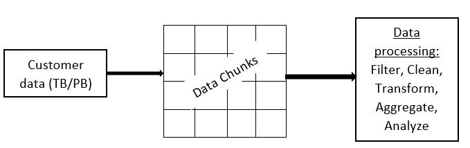
So, even if you lose data on one node, the data will be available on other nodes due to replication. Data processing happens on different nodes parallelly, making Spark faster.
Why Use Spark for Big data Analytics?
Some important factors to prefer Spark for Big data analytics (data science with Spark) are ease of use, speed, efficient handling of large sets of data, iterative processing, real-time processing, graph processing, storage and analysis, and machine learning. But the question is, why do we need Spark when we already have Hadoop? As we discussed before, Hadoop is suitable only for batch processing and not for real-time data processing. Spark, on the other hand, can do both. Further, MapReduce is a bit complicated, especially for beginners, and it is slow as well. Also, MapReduce involves too many I/O operations (at each step). Spark is easy to use and offers faster processing as it stores data in the memory. This is done through RDD. Let's know more about it.
RDD
RDD stands for Resilient (or reliable) Distributed Data. It splits data into chunks on the basis of a key and distributes it among the executor nodes. RDD supports transformations and actions. There are very few I/O operations, and the data sits in the memory. Spark can handle data even with less memory. Some properties of RDD are:
- Lazy evaluations,
- In-memory computations, and
- Immutability (data values can’t be changed once committed).
Introducing PySpark: Spark Python API
As we have mentioned before, PySpark is the Python API for Spark that helps us work with RDDs using the Python programming language. PySpark is a great API to perform computations and analyze voluminous datasets. PySpark is also compatible with Python, R, Scala, and Java. It provides fast processing, a powerful caching mechanism, and disk persistence. Also, it is dynamically typed, and can easily perform real-time computations. Another advantage of using the Spark Python API is that it has powerful data science libraries to perform data analysis and data visualizations. Let us see some action and transformation functions performed by PySpark, which are useful for data science. The RDD performs action and transformation functions. First, we have to load the dataset into RDD:
RDDdata = sc.textFile(<path of the data file>)
Here, sc is the SparkContext.
Action operations
Action operations perform computations on the dataset. Some common action operations are:
- take(n) : This function displays the specified number of elements (n) from the RDD file. For example, RDDdata.take(10) will display an array of the first 10 elements of the dataset. Suppose a list has the elements List(1,2,3,4,5), and we call the take function with parameter 3. Then the result will be 1,2,3.
- count() : Count returns the number of elements in the RDD.
- top(n) : Displays the top n elements from the dataset.
Transformation operations
Transformation operations create an entirely new RDD or modify elements of an existing RDD using the function. Some examples of transformation functions are:
- Map transformation : If you have to transform each element of the RDD, you can use map transformations. A good example can be transforming the entire dataset into an upper case using the upper() function.
-
Filter transformation : These are applied to remove elements from the dataset. These elements are known as stop_words, and you can define your own set of stop words.
Many domains use PySpark, including healthcare, e-commerce, and finance.
Data Science with Spark (Tasks Performed Using Spark)
Now that we are familiar with Spark and how its components, like SparkContext and RDD, work, next we will move on to SparkSQL using Python. We use it for data science tasks like text mining, categorization (tagging), pattern extraction, sentiment analysis, and linguistics. We will discuss some of the common task functions using Dataframes.
Data Cleaning and Analysis
Data cleaning can be done using both Data Frames and SQL. Dataframe has more functions for cleaning and is more efficient. Although Spark Dataframe is similar to pandas (the popular data science library for Python), it is more efficient and distributable.
Using Spark Dataframe
The data is chunked into multiple nodes and runs in a distributed manner, so memory consumption is less. Also, this makes the computations less expensive. Some common Spark Dataframe functions are:
- table() : Creates a Dataframe. For example, val dfr = spark.table("dataset").
- show() : Shows all the records in the Dataframe.
- describe() : Gives descriptive statistics, like mean, count, and max for the numeric columns.
- select() : Selects particular columns or SQL expressions. Example: dfr.select(“employee_name”);
- cache() : Persists the DataFrame into the default storage level (memory/disk). Creates temporary tables only for the particular session.
- corr() : Finds the correlation between two columns. Example, dfr.stat.corr(‘age’, ‘weight’)
- groupby() : Groups the results by a particular column. For example, if we want to see the number of students belonging to each department, we can use groupby(). Example, dfr.groupby(‘department’).count.show();
- stat.freqItems() : Gives the frequent items in the dataset. For example, what are the main reasons people state for not exercising in their age groups? This function also accepts a decimal, which denotes the frequency of occurrence. Example, dfr.stat.freqItems([‘reasons’, ‘age_group’], 0.4)
- approxQuantile() – Saves cost and execution time. We can specify the amount of error that is acceptable for us so that the execution time is as less as possible. Since the dataset is distributed, we cannot obtain the quantile directly, so we find it approximately.
- coalesce() : Used for obtaining non-null values. If a column has many null values, this function merges with/creates a new column with non-null values. Example, if column_1 has values [1,2,null,4,null] and column_2 has values[1,2,3,4,5], both will be combined to form a single column (column_1, column_2 or a new column) which will have non-null values as [1,2,3,4,5].
There are many other functions for basic statistics like aggregate (agg), average (avg), maximum (max), etc. Check the complete list on the official DataFrame documentation page.
Using SparkSQL
SparkSQL also has similar functions for cleaning. We can use regex functions to extract and transform data, for example, removing ‘years’ from ‘3 years’ or '%' from '99%'. This is done to remove outliers and missing values. Example:
dfr.withColumn(“employee_name”, regexp_replace(col(“employee_name_new”, “Mr”, “”));
In the above code, we are selecting the employee_name column and then removing the title ‘Mr’ from the name and replacing it with blank spaces. Now, observe this code:
dfr.withColumn(“age”, regexp_extract(col(“age_new”), \\d+, 0));
This extracts only the digit (d) part of the age, removing any other text like years or months, etc. For effective cleaning, each column that has a null value, should be individually analyzed and fixed to remove the null values. This can be done using the command:
df_sel.select([count(when(isnan(c) | col(c).isNull(), c)).alias(c) for c in df_sel.columns]).show()
where c is the counter that loops through each column value. In SQL, we can do the same using the count function as:
select count(*) from table_name where column_name is NULL;
Finding Patterns in Data
The main aim of cleaning is to find similarities and patterns in the data so that only the required features can be kept in the clean data set. Suppose a column has a lot of null values. In such a case, we can check the other columns of the table and see if there is a pattern. For example, whenever it rains, the demand for ice cream and brownies is null. As per our data, this happens almost all the time. In that case, we can merge the icecream_sales column with some other column, like brownie_sales, which has a similar value, using the coalesce() function.
Exploratory Data Analysis
Exploratory Data Analysis (EDA) is an important step that determines whether our analysis is going in the right direction or not. It is the primary analysis of data to find patterns, trends, and other data features on the structured (cleaned) data.
EDA and Visualization
EDA also involves data visualization, i.e., viewing the patterns and data features in a graphical form to obtain a better view. Suppose we want to know the cities having a temperature of more than 45°C in the US during April. For that, we can filter the data using the filter() function:
dfr.filter(dfr.temperature > 45).show()
The filter() function is most commonly used to remove or replace missing values from the dataset. What if we wanted to sort the data based on the marks obtained by students in the current academic year? In such a case, we can simply use the orderBy() function:
dfr.orderBy(dfr.avg_marks).show(10)
Earlier, we have seen the
freqItems()
method. It achieves the same purpose but shows some more statistics other than
orderBy()
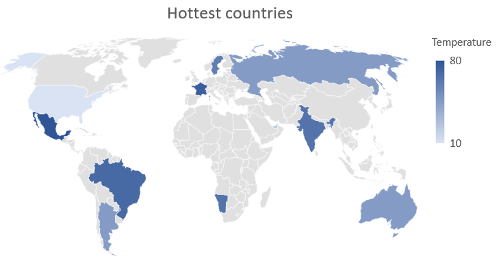
. Now, let us look at how to perform some visualizations. The most popular tool for this is Databricks, which was developed for collaborative data science. Once the data is cleaned, it is very easy to perform EDA using Databricks. It gives easy UI options for you to create visualizations based on the parameters you select. For example, if we need to see the hottest countries in the world in April, we can simply create a map with the average temperatures:
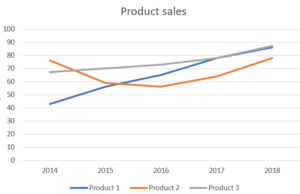
 Same way, if we want to compare the sales of 3 different products over a period of 5 years, we can use a line plot as shown below:
 Similarly, we can create any visualization, including histograms, bar charts, area charts, and scatter plots. We can also create customized plots, using the key columns, groupings, and values (aggregate functions). Learn more about
Databricks from this short video.
Similarly, we can create any visualization, including histograms, bar charts, area charts, and scatter plots. We can also create customized plots, using the key columns, groupings, and values (aggregate functions). Learn more about
Databricks from this short video.
Conclusion
That wraps up this article about data science with Spark. Here, we have learned the basic functions used to perform data cleaning and data processing using PySpark, the Spark API for Python. We also understood the basic architecture and components of Spark and how it is better than Hadoop. The main advantages of Spark are its speed, data parallelism, distributed processing, and fault tolerance. Learn more about data science and machine learning . People are also reading:
- Best Data Analytics Tools
- Data Visualization Tools
- Data Science vs Machine Learning
- Decision Tree in Machine Learning
- Data Analysis Techniques
- Data Science vs Artificial Intelligence
- What is Unsupervised Learning?
- Data Science Interview Questions and Answers
- What is Supervised Learning?
- SQL for Data Science


Leave a Comment on this Post