

Whenever there is a question that has an answer in yes or no, true or false, or we have to choose one out of many options, we immediately tend to make a decision. For example, “Do you want milk now?”, “Should I take up this course or some other one?” etc. A computer can do that too, provided we train it using some algorithms. A decision tree in machine learning is used for this purpose. Decision trees can be used for both classification and regression problems.
Classification Algorithms
Classification algorithms help us categorize data into distinct classes so that we can assign a label to each class. These algorithms are widely used for handwriting recognition, speech recognition, biometric identification, and more. There are two types of classifiers:
- Binary classifier – These classifiers have only two distinct outcomes (classes). For example, whether an email is spam or not, whether a child likes milk or not, whether a student passes or fails.
- Multi-class classifier – Classifiers having more than two classes or outcomes are multi-class classifiers. Colors of various objects and classification of different songs based on moods are examples of multi-class classifiers.
Let us take a simple dataset to show a classification problem:
| Shape | Color | Vegetable |
| Round | Green | Cabbage |
| Oval | Green | Cucumber |
| Oval | Orange | Carrot |
| Oval | Purple | Brinjal |
| Round | Yellow | Squash |
| Oval | Yellow | Potato |
| Round | Red | Tomato |
The shape and color are called attributes of the dataset, and the vegetable is the label. For example, if the input is oval and green, then the answer will be cucumber as per the dataset. Now, if a new input is given with the attribute oval and yellow, a decision tree can ask questions like is the shape oval or is the color yellow, and accordingly, label it as Potato.
Decision Tree in Machine Learning
The decision tree in machine learning is an important and accurate
classification algorithm
where a tree-like structure is created with questions related to the data set. The answer to a question leads to another question, which leads to another, and so on until we reach a point where no more questions can be asked. How the questions are asked and what attributes are chosen is decided based on some calculations that we will discuss in this article later. A simple decision tree in
machine learning
looks something like this:
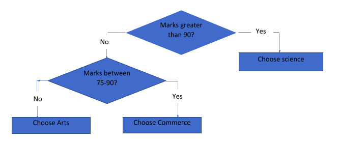 This is a simple tree where a student can decide the subject she can take up based on the marks. Thus, ‘marks’ is the main attribute here, and we decide the questions to be asked based on this attribute. The decision tree is easy to understand and can be represented in a diagrammatic manner, making it easy to visualize. Also, a decision tree can handle quantitative as well as categorical data, and it is widely used for predictive data analysis. But how do you decide what questions to ask? To answer this, let us create a decision tree for the above classification dataset that we have:
 The next question will be based on the answer to this question. Thus, the questions are based on the attributes of the dataset. Now, how do you decide which should be the best attribute? This is where machine learning algorithms come into the picture. We decide the attribute based on how well the decision tree can be split and unmixed using the attribute. Before getting into details of this, let us understand the types of decision tree algorithms and important terms associated with decision trees.
Types of Decision Tree Algorithms
We can create a decision tree using many different algorithms. The most popular algorithms are:
- ID3 (Iterative Dichotomiser 3) – ID3 algorithm iterates through each attribute of the dataset to find the entropy and information gain of the attribute. The attribute with the highest information gain is then taken as the root node that splits the decision tree.
- CART (Classification And Regression Tree) – This algorithm can be used for classification (category) as well as regression (numeric) problems. It is a binary decision tree where the root node is split into two child nodes by asking a set of questions. The questions should resemble the dataset. Also, the answer to each question further splits the node, and the next question can be asked.
- CHAID (CHi-square Automatic Interaction Detection) – This decision tree technique is used for the detection of interaction between two or more variables, classifications, and predictions. It is mostly used for targeted marketing to certain groups and predicts how they respond to different scenarios.
In this article, we will create a decision tree from scratch and understand the terminology associated with it. So, let us familiarize ourselves with the important terms that we will be using in constructing our decision tree.
Important Terms
Some important terms used in the decision tree algorithm are:
Gini Index
It is an index used to quantify the amount of uncertainty.
Entropy
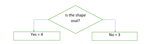
This is the measure of the impurity in the dataset. If all the labels and items are the same, the impurity is zero. For example:
 However, if there are mixed items in the dataset, the probability of the label and item being the same becomes less. Such a dataset will have a non-zero impurity value. For example:
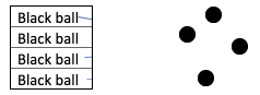
 This means that if the degree of randomness in the data is high, impurity ? 0. However, if data is pure or impure (i.e. no randomness), impurity and thus entropy are both zero. Suppose we split our decision tree based on a question, "Is the ball orange?" There could be two answers to this question, yes or no. In a dataset with 100 such rows, there could be many orange balls and balls of other colors. Suppose there are 50 orange balls and 50 balls of some other color. Then, there would be 50 yes and 50 no as answers for the question. For a situation like this:
where n(yes) = n(no), entropy will always be = 1.
In general, the entropy of a sample S in a dataset can be calculated with the following formula:
| Entropy(S) = -P(yes)log2P(yes) – P(no)log2P(no) |
Information Gain
This value decides which attribute should be selected as the main decision node based on how much information it gives to us. We measure the reduction in entropy for the sample S to get the information gain: Information gain = Entropy(S) – Information Taken, where “information taken” is calculated as {Weighted average x Entropy (individual features)} Thus,
| Information gain = Entropy(S) - {Weighted average x Entropy (individual features)} |
Chi-Square
It is used to find the importance of the difference between the parent node and subnodes.
Variance Reduction
It is used for regression problems (continuous variables) where split with lower variance acts as the criteria for splitting the sample.
Decision Tree Diagram Terminology
Some important terms related to the decision tree diagram are:
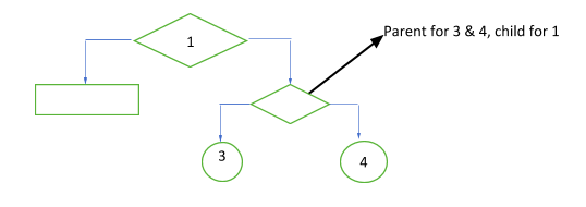
- Root node – It is the first node of the decision tree, the point where the tree starts. It represents the entire sample.
- Leaf node – It is the last node of the decision tree. After this, no more segregations are possible.
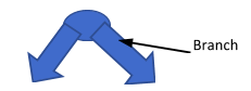
- Subtree/branch – When we split the node or tree, we get these.
- Splitting – It is the process of dividing the nodes into subparts based on a question or condition.
- Pruning – It is the removal of unnecessary, excess, or unwanted nodes of the tree. Pruning helps in avoiding the problem of overfitting.
- Parent/Child – Except for the root node, all the nodes of a decision are called child nodes. Some nodes can be both parent and child when there are multiple branches. The root is always the parent node.
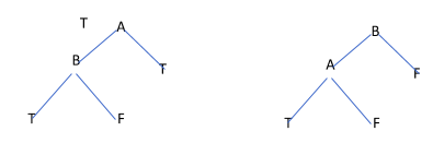
 Try these examples to create decision trees and understand each part of the diagram:
- A person will buy a certain product during shopping.
- A person will diagnose positive for heart disease.
- Check if an email is spam or not.
Building a Decision Tree in Machine learning
We know how to create a tree and split the nodes, but one question remains unanswered:
“ How to decide the best attribute?”
We will focus on answering this question by using the following data set. In the below dataset, 3 attributes will be used to answer the question, “Should I eat a banana today?” Yes, you are right! That’s a simple problem for our brain, but how does the computer do it? Let's know.
| State of the banana | Health of the person | Weather | Eat or not? |
| Raw | Good | Sunny | No |
| Ripe | Cough | Rainy | No |
| Ripe | Wheezing | Sunny | No |
| Ripe | Cough | Sunny | Yes |
| Ripe | Wheezing | Rainy | No |
| Ripe | Good | Rainy | Yes |
| Ripe | Good | Sunny | Yes |
| Raw | Good | Rainy | No |
Calculating the Entropy
Take some time to understand the dataset. If the banana is ripe, but the person who wants to have it has wheezing, he/she should not eat it. If the banana is ripe, the person who wants to have it has a cough, but if the weather is sunny, he/she can eat it. Same way, others. There are 8 instances in our ‘Banana’ dataset. There are 5 No values and 3 Yes values. This means the probability of getting No as the answer is 5/8 and Yes is 3/8. Let’s calculate entropy for this example using the formula we mentioned above: Entropy E(S) = -(3/8)*log2(3/8) – (5/8)*log2(5/8) = -3/8*(-1.415)-5/8*(-0.678) = 0.95 If we had had an equal number of Yes and No, the entropy would have been 1.
Deciding the Best Attribute
We have three attributes, namely state, health, and weather. Which attribute should be our root node? To decide this, we need to know the information gain that each attribute can give us. Whichever node gives the maximum information gain wins! So, let calculate the same using the formula we mentioned above! The above formula should be applied to each attribute to calculate the information gain.
Attribute 1 – State
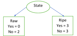 Let's start with the state attribute. To calculate information gain, we need first to calculate information taken, which is again calculated by multiplying the weighted average with the entropy of individual features values. In this case, the values are ripe and raw. For a totally impure or pure set (no randomness), the entropy is 0, as we have seen before. Therefore, Entropy (Raw) = 0 because there is no yes, only no. If we calculate this using the formula, we will get the same result. Entropy (Ripe) = 1 because of the equal number of yes and no. Using the formula, we can calculate this as -(3/6)*log2(3/6)-(3/6)*log2(3/6) = 1. Information taken, IT(State) = 2/8*Entropy(Raw) + 6/8*Entropy(Ripe) = 2/8*0 + 6/8*1 = 0.75 Information gain, IG(State) = E(S) – IT(State) = 0.95-0.75 =
0.20
Let's start with the state attribute. To calculate information gain, we need first to calculate information taken, which is again calculated by multiplying the weighted average with the entropy of individual features values. In this case, the values are ripe and raw. For a totally impure or pure set (no randomness), the entropy is 0, as we have seen before. Therefore, Entropy (Raw) = 0 because there is no yes, only no. If we calculate this using the formula, we will get the same result. Entropy (Ripe) = 1 because of the equal number of yes and no. Using the formula, we can calculate this as -(3/6)*log2(3/6)-(3/6)*log2(3/6) = 1. Information taken, IT(State) = 2/8*Entropy(Raw) + 6/8*Entropy(Ripe) = 2/8*0 + 6/8*1 = 0.75 Information gain, IG(State) = E(S) – IT(State) = 0.95-0.75 =
0.20
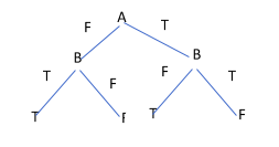
Attribute 2 - Health
Now, let’s calculate the information gain for the next attribute, i.e. health. Consider the following decision tree:
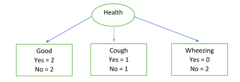 E(Health = Good) = 1 (Guess, why?) E(Health = Cough) = 1 E(Health = Wheezing) = 0 Information Taken, IT(Health) = 4/8*1 + 2/8*1 + 2/8*1 = 0.75 IG(Health) = 0.95 – 0.75 =
0.20
E(Health = Good) = 1 (Guess, why?) E(Health = Cough) = 1 E(Health = Wheezing) = 0 Information Taken, IT(Health) = 4/8*1 + 2/8*1 + 2/8*1 = 0.75 IG(Health) = 0.95 – 0.75 =
0.20
Attribute 3 - Weather
The last attribute is Weather. So let us calculate the IG for that:
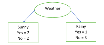 E(Sunny) = 1 E(Rainy) = -1/4*log2(1/4) – ¾*log2(3/4) = 0.5 + 0.31125 = 0.81125 Information Taken, IT(Weather) = 4/8*1 + 4/8*0.81125 = 0.905625 = 0.90 Information Gained, IG(Weather) = 0.95 – 0.90 =
0.05
E(Sunny) = 1 E(Rainy) = -1/4*log2(1/4) – ¾*log2(3/4) = 0.5 + 0.31125 = 0.81125 Information Taken, IT(Weather) = 4/8*1 + 4/8*0.81125 = 0.905625 = 0.90 Information Gained, IG(Weather) = 0.95 – 0.90 =
0.05
Comparing the 3 Values
When we compare the 3 values, we note that IG(Health) and IG(State) have better information gain as compared to IG(Weather). Since both IG(Health) and IG(State) are equal, we can use any of them as the root node to create the decision tree. Here, we are taking the Health attribute. By doing so, our decision tree should look like this:
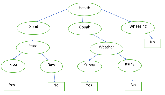 The last nodes with the yes and no values are the leaf nodes because the decision tree ends there. One last thing on this decision tree, and then we will move on to how the computer internally performs the logic of getting the yes and no.
Pruning the Tree!
We can prune this tree by removing all the no values so that we get a compact decision tree. By doing so, we will get this:
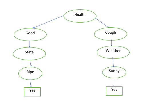 We can represent this using Boolean values. For example, if health is good AND state is ripe, we can eat the banana. Same way, if we have a cough but the weather is sunny, we can eat. However, if you have a cough OR the weather is rainy, we cannot eat the banana. This means we can represent a decision tree in machine learning using OR, AND, NOT, and XOR operators. AND
| A | B | A AND B |
| F | F | F |
| F | T | F |
| T | F | F |
| T | T | T |
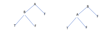 OR
OR
| A | B | A OR B |
| F | F | F |
| F | T | T |
| T | F | T |
| T | T | T |
 XOR
XOR
| A | B | A XOR B |
| F | F | F |
| F | T | T |
| T | F | T |
| T | T | F |
 In the above case, we have only two attributes, A and B. If we have more attributes, like C, D, E, and so on, the tree will need an exponential number of nodes. For n attributes, the number of nodes will be approximately 2^n or 2n. This is how to create a perfect decision tree in machine learning.
Decision Tree Boundary
The goal of a decision tree in machine learning is to create a boundary that separates the data into linear, rectangular, or hyperplane representations based on the qualities of the data. The decision boundary forms as each data point settle into space in the X-Y coordinates. Let’s take a simple example. Suppose there are these numbers in a dataset, {10, 12, 15, 16, 27, 56, 67, 45, 89, 34, 76, 95, 23, 90}. Consider each of the numbers as a data point. When we get a new number, say, 65, where should it go? Our decision tree asks the question: Is the number greater than 50?
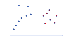 The new number 65 thus goes to the red group where all the numbers greater than 50 are placed. The dashed line is the boundary that is created when the decision tree splits the data. If there are more variables, the plane will change accordingly.
When to Use a Decision Tree in Machine Learning?
We can use decision trees when:
- We need an algorithm that can be easily viewed and represented.
- Nonlinearity is high.
- It is required to define a complex relation between independent and non-independent variables.
Python Code Implementation of a Decision Tree in Machine Learning
To build a decision tree in machine learning using Python, we use the scikit-learn library. Let us import the required libraries to start with:
#Importing libraries
import pandas as pd
import numpy as np
from sklearn.tree import DecisionTreeClassifier
from sklearn.model_selection import train_test_split
The next step is to get the data. We can create the data or load it from the existing datasets:
training_data = [[‘Round’, ‘Green’], [‘Oval’, ‘Green’], [‘Oval’, ‘Orange’], [‘Oval’, ‘Purple’], [‘Round’, ‘Yellow’], [‘Oval’, ‘Yellow’], [‘Round’, ‘Red’]]
label_data = [‘Cabbage’, ‘Cucumber’, ‘Carrot’, ‘Brinjal’, ‘Squash’, ‘Potato’, ‘Tomato’]
We have fewer data in our dataset. However, you can expand to add more rows or use an existing dataset that comes with scikit-learn. Let’s split the data into training and testing sets:
X_train, X_test, y_train, y_test = train_test_split(training_data, label_data, random_state = 47, test_size = 0.25)
To find the information gain, we need to find the entropy, which will be the criteria for splitting the decision tree, as we saw earlier in our banana example. For this, we will need to get the DecisionTreeClassifier from the scikit-learn library (we have already imported it):
data_classifier = DecisionTreeClassifier(criterion = 'entropy')
To get more accuracy, we can set the minimum number of samples along with the criterion as min_samples_split = n, where n will be the minimum number of data samples required to split the node. We can do this if the accuracy of the training data is more than the accuracy of the test data. Next, we use the classifier to train the data:
data_classifier.fit(X_train, y_train)
Now, we use the algorithm to predict test data. We will have to import the accuracy metric from the sklearn.metrics library:
y_pred = data_classifier.predict(X_test)
from sklearn.metrics import accuracy_score
print('accuracy score - training data: ', accuracy_score(y_true=y_train, y_pred=data_classifier.predict(X_train)))
print('accuracy score - test data: ', accuracy_score(y_true=y_test, y_pred=y_pred))
Conclusion
We have covered the basics of a decision tree in machine learning and how to create one from scratch by taking a simple example. You can try doing the same for the other examples we have mentioned in our article. The decision tree is the most appealing algorithm for visualizing what is happening at each step and can handle categorical as well as numeric data. Decision trees are resistant to outliers and require very little pre-processing. However, they are prone to overfitting and can create a high bias if some classes are more dominant. Nonetheless, by using decision trees, we can establish and understand complex relationships between dependent and independent variables as well. People are also reading:
- ML Books
- Best Machine Learning Interview Questions
- Best Machine Learning Frameworks
- How to become a Machine Learning Engineer?
- Machine Learning Projects
- Classification in Machine Learning
- AI vs. ML vs. Deep Learning
- Machine Learning Applications
- Machine Learning Algorithm
- Data Science vs. Machine Learning


Leave a Comment on this Post