Introduction to Classification Algorithms

There are 3 main types of machine learning algorithms; supervised, unsupervised, and reinforcement. Classification is a type of supervised learning algorithm in which incoming data is classified or labeled based on past data. The algorithm is trained by feeding it with different types of labeled data that can be categorized into different outcomes. For example, we can train a model to identify cats, dogs, and horses in the data fed based on features like eyes, color, size, and shape. Once the model is trained, it can categorize a new set of data into the same categories’ cats, dogs, and horses.

Classification Algorithms Scenarios

Different machine learning algorithms can solve different types of problems. Sometimes more than one model (algorithm) is applied to the data to get the final solution. Some typical scenarios where classification algorithms are used are:

Detecting if an email is spam or not spam.
Identifying the gender of a person on the basis of certain features (like hair length and body structure).
Grouping similar items together – for example, the same type of files, same fruits, the same type of news items, the genre of music and movies, etc.
Identifying if a user will buy particular accessories with a product.

There is no particular rule that states what type of algorithms should be used for a particular problem. Generally, data scientists and machine learning engineers perform controlled experiments to determine the most suitable algorithm for a particular task. If we were to represent a classification algorithm mathematically, it would be a mapping function from the input variable A into output variable B, where B = f( A ).

What are Classification Algorithms?

Classification algorithms classify or categorize items based on their similarities. The model is trained using a set of data for which the output is already known. Once the model is trained and has good accuracy, new data is supplied for testing and evaluation. The outcomes are called a target class or class label. For example, if the model has to classify the following fruits based on their shape, size, and color, the target classes will be each of the fruits. Mixed fruit basket

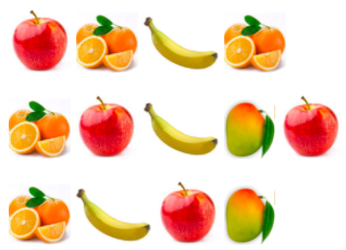
Mixed fruit basket: (Image source: Wikipedia)

When we classify this, we will get the result as: classify Mixed Veg Fruit

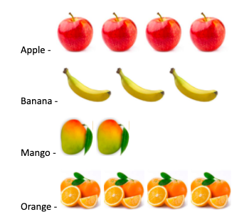
This labeling and classification of data can be done using many algorithms. Before getting into that, let us explore some common terminologies in classification.

Important Terms in Classification

Feature – A feature is a measurable property. For example, height, length, and size are features.
Classifier – It is an algorithm that correctly maps the input into one of the categories. For example, linear classifier and naïve Bayes classifier.
Label – Names assigned to the output categories are labels. For example, Apple and Orange are labels for fruits.
Class – It is the instance into which the problem is categorized. For example, in the problem of identifying if an email is a spam or not spam, the target classes are ‘spam’ and ‘not spam.’

Types of Classifications

There are different types of classification algorithms:

1. Binary Classification

Binary classifications have two target labels. These are usually the outcomes of ‘yes’ or ‘no’ to a problem. For example, a person will buy a particular course or not, an email is spam or not, a patient has a particular disease or not, a product passed a quality test or not. Remember that binary classification is one of the below:

Some of the popular algorithms used for binary classification are – k-NN, decision trees, logistic regression, SVM and Naïve Bayes. Algorithms like logistic regression and SVM support only binary classification. To test the accuracy of each of the above classifier algorithms, we use various methods like confusion matrix, ROC curve, cumulative gain, positive and negative rates, lift chart, binary classification tests like classification accuracy, error rate, sensitivity, and specificity.

2. Multi-class Classification

If a task has more than 2 class labels, it comes under multi-class classification. Unlike binary classification, there is no yes or no outcome here; instead, classification is done among a set of known classes. A data sample can belong to only one particular class. For example, an animal can be a lion or a tiger but not both at the same time. Multi-class classification is the most commonly-used classifier of all. Some of its use-cases are:

Filtering out particular words in a text (email, document, resume, etc.) to identify phishing emails, relevant keywords, etc.
Identifying the rating (A, U, U/A) of a movie based on the tags and content.
Helping businesses predict the next set of products that a user might like to buy on the basis of their current purchases and preferences.
Handwriting recognition, image classification, and intent classification.

The most popular algorithms that we use for this type of classification are kNN, decision trees, random forest, gradient boosting, Naïve Bayes, and neural network classifier. We will learn about each of these later in this article.

3. Multi-label Classification

In multi-label classification, a data sample can belong to many labels. For example, a person can be adept in history as well as physics, or love both comedy and horror genres, a piece of news can belong to both sports and music category and so on. Multi-label classifiers require knowledge of the correlation between the various classes and can be considered as the generalization of the multi-class classification. The most common classifiers that we use here are the modified versions of k-NN, decision trees, kernel methods and neural networks. The scikit-learn package helps in implementing multi-label algorithms in Python.

4. Imbalanced Classification

In an imbalanced classification, the number of examples in each class is not equally distributed. It is a type of binary classification, where most of the examples belong to a class A which is normal, and some (less) belong to class B, i.e. not normal. Some typical scenarios where imbalanced classification is used are outlier and fraud detection, medical diagnosis tests. Decision trees, SVM and logistic regression are commonly used algorithms. Performance metrics can be calculated using precision, recall, f-measure.

Types of Learners

There are 2 types of learners in a classification algorithm:

Lazy learners : These learners perform classification only after receiving the testing data. These learners invest more time in predicting and less time in training. K-nearest neighbors and case-based reasoning are lazy learning algorithms.
Eager learners : Eager learners do not wait for testing data. They work on training the model, thus spending more time on training, and reducing the time spent on prediction. Decision trees, artificial neural networks and Naïve Bayes are eager learning algorithms.

Popular Classification Algorithms

We have already described some of the above algorithms in our article on supervised learning , you can check it out if you wish to go into the details. Let us now explore more about the classification algorithms.

1. k-NN

k-NN refers to k-nearest neighbors. In this algorithm, finding the category of the new data sample depends on determining its nearest neighbors. If the data point has more neighbors of a particular class, the data point is assigned the same class. A simple diagram to illustrate the same is as follows: K-NN

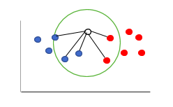
In the above picture, for the white circle, there are 3 blue neighbors and 2 red neighbors. As 3 > 2, we will classify the new circle in the blue category.

2. SVM (Support Vector Machines)

In SVM, we mark each data item (sample) as a point in n-dimensional space, where n is the number of features. Each feature represents the axis coordinate. To classify the items, a hyperplane is constructed that best separates each class of data items. Linear hyper-plane: In this case, we can classify the data items linearly, i.e. within a straight line. Sometimes, there might be an outlier (as shown below), however, SVM ignores the outliers. 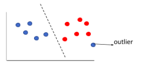Non-linear hyper-plane: If you have the below plot of data items, how would you classify them? 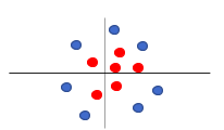For this, we have to create another dimension and represent the data in the new dimension. If we look at the data from a different dimension, below is how it will look like (Think of the below view as the view of the same data from the left or right side and the above view as the top view of the data.): 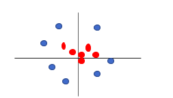If we now classify the data, we can see that the hyperplane is a circle. 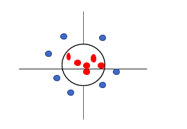This method is also called the kernel trick, where a feature (axis) is added manually to get the best hyperplane, thus converting a lower-dimensional plane into a higher-dimensional plane.

3. Decision Tree

As the name suggests, decision trees split the data into smaller subsets to form a tree-like structure. The nodes split on the basis of the answer to a question. For example, the question, “Will it rain tomorrow?”, can have 3 possible answers; yes, no or maybe. Based on these 3 answers, the data can be split into smaller subsets. We form further questions on the basis of these answers, and the tree keeps splitting until no splits are possible. Check out our article on the decision tree in machine learning for an in-depth analysis of this classification algorithm.

4. Naïve Bayes

Considered to be the easiest among the classification algorithms, Naïve Bayes is also the most popular of all. It is based on the Bayes theorem, which uses probability and conditional probability to predict the class of datasets that are unknown. For simplicity, the ‘Naïve’ Bayes assumes that the presence of one feature is independent of other features in the dataset. The Bayes theorem is as follows: P(A|B) = P(A)*P(B|A)/P(B) where,

P(A|B) = posterior probability of the target A, given B (attributes) are true.
P(A) = prior probability of class A.
P(B|A) = likelihood of or probability of the predictor B given the class A is true.
P(B) = probability of the predictor B (attributes).

Let us understand Naïve-Bayes with a simple example. Say, we have all the face cards of a pack. What is the probability that we get Q of the spades as the first card after a shuffle? We know that we have only the face cards and that there are 16 face cards in a pack. Therefore, the probability of getting a ‘Q’ out of the face cards, i.e. P(B) = 4/16 = ¼ The probability of getting a spade, i.e. P(A) = 4/16 = ¼ Now, the likelihood of getting a spade if we know that the card is Q, i.e. P(B|A) = 1/4 Therefore, the posterior probability that the first card we pick will be a Q of spades, P(A|B) = (1/4*1/4) /(1/4) = 1/4 This is an excellent simple example to understand how probability works. Some of the real-time problems that are solved by the Naïve Bayes algorithm are:

Text classification,
Sentiment analysis,
Filtering spam messages, and
Recommender systems (along with collaborative filtering).

In Python, the scikit-learn package offers 3 types of Naïve Bayes models; Gaussian, Bernoulli (Binomial), and Multinomial.

5. Logistic Regression

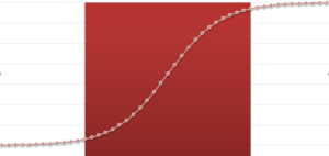
As the name suggests it has something to do with regression. The logistic regression algorithm is a popular algorithm for binary classification problems (binomial logistic regression). There could be more than 2 classes as well, which we call multinomial logistic regression. The core of this classification algorithm lies in using the logistic or sigmoid function , which indicates exponential growth in the data and maps all the real values into a value between 0 and 1. If we plot the data, we will get an S-shaped curve, the function being p(x) = 1/(1+e-(?x)). The curve of a logistic regression also flattens out near 0 and 1. As the input gets positive and large, the output becomes closer to 1. On the contrary, if the input is negative and large, the output goes closer to 0. Logistic regression is considered to be a generalized form of a linear model, which is because the decision boundary (of classification) is linear. The model produces some probabilities, on the basis of which the classification is done. A threshold value is set that decides the outcome. A simple example is to predict whether an employee would get the job or not. Since probability always lies between 0 and 1, typically the threshold is set at 0.5 (half), i.e. if the probability is greater than 0.5, the employee is more likely to get the job. This probability comes out on the basis of a combination of factors, let’s say, confidence, communication ability and subject knowledge. After applying the logit (logistic) function, we would get a plot in the shape of S for the given data, as shown below: Logistic regression

6. Random Forest

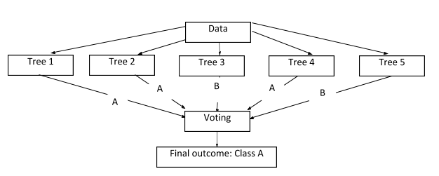
The random forest classification algorithm creates decision trees. The more the number of trees, the stronger the algorithm becomes. Random forest eliminates the issue of over-fitting that could occur while using a single decision tree. In this algorithm, the data is split into smaller sets and decision trees are constructed from these smaller samples. Each decision tree gives an outcome. If there are n decision trees, we get n outcomes. Finally, we use voting to decide the best-predicted value, which then becomes the outcome. It is a type of ensemble method for machine learning. Random forest

7. Gradient Boosting

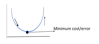
GBM is another ensemble algorithm that generates a prediction model by combining weak learning models, mostly decision trees. By combining the weak models, we get a more robust model. This is done by optimizing the mean squared value (i.e. the average of the square of the difference between targeted and predicted values from a sample). By combining the MSE (Mean Squared Error) of each weak model, the overall MSE value reduces in the final model. GBM uses 2 direction vectors, namely, the residual vector and the sign vector. Also, it uses the gradient descent optimization technique to find the minimum error value by moving in the direction of the steepest descent. Think of this function similar to you going down a hill through a steep path till you reach the bottom, from where you can only go upwards. Gradient boosting

8. Neural Networks

Neural networks are deep learning techniques that try to mimic the human brain in making decisions and predicting outcomes. In such a network, each neuron connects to many others using connection links. The connection links contain information about the input signal (neuron). These are called weights and are responsible for either activating or inhibiting the input signal. The output is a result of the processing of input using an activation function. Thus, the 3 layers of an artificial neural network are:

The input layer (Collects the input and gives a pattern to the hidden layers).
Hidden layers (Where the input is processed. There can be n hidden layers).
Output layer (Collects and transmits the output).

The hidden layer consists of aggregation and activation functions. Following is a representation of the entire ANN structure: Neural networks

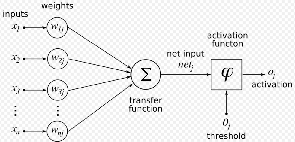
Image source : Wikimedia

Here, the transfer function is the summation function, ?xnwnj and activation oj is the output. ANN follows the iterative learning process where rows are presented to the network one at a time, and weights are adjusted every time on the basis of the errors of the previous output. The weights keep adjusting to achieve the desired accuracy in predicting the correct class of the input data. Neural networks can classify entirely new data patterns that have not been trained as well. The several types of ANN include Perceptron, convolutional neural network, LSTM, shallow neural networks, recursive neural networks, and modular neural network. Neural networks find use in NLP (Natural Language Processing), text classification, part-of-speech tagging, paraphrase detection, language generation, document summarization, targeted marketing, and medical diagnosis.

Applications of Classification Algorithms

Classification algorithms have a wide range of applications. Some of the most critical and practical applications of classification algorithms are:

Speech recognition.
Handwriting detection.
Document classification, image and video classification.
Biometric identification.
Recommender systems.
Internet traffic inception.
Click-stream analysis (i.e. to predict if a user will buy certain products on the basis of their past clicks and purchase history).

Conclusion

That sums up explaining one of the types of supervised learning algorithms, i.e. classification algorithms. It includes many classifiers like SVM, logistic regression, and random forest. As this is only an introductory article, the actual implementation of algorithms (code) is out of scope here and thus, we will cover it in detail in separate articles. To summarize:

We categorize data into several classes using different classifiers.
A classification algorithm is a type of supervised learning mechanism.
The algorithm makes conclusions and predictions based on the values received through model training.
The most popular classification algorithms are SVM, Random forest, Naïve Bayes, decision tree, GBM, neural networks, and logistic regression. We can implement each of these using the scikit-learn package in Python.
Different types of classification algorithms are binary, multi-class, multi-label and imbalanced.

People are also reading:

Introduction to Classification Algorithms

Classification Algorithms Scenarios

What are Classification Algorithms?

Important Terms in Classification