Introduction to Classification in ML
Classification is one of the most important types of supervised learning algorithms. In a supervised learning algorithm, the machine learns from a supervisor to give output for new observations or a new set of data. In classification, data is categorised into several classes based on known labels (classes, targets or categories).
The machine has a set of data for which the expected output is known. The machine trains with this data and builds a model. Then a new data set is given to the machine to predict the class of each data point and test the accuracy of the model.
Classification can be performed on structured as well as unstructured data. Some simple examples are – identifying an email as spam or non-spam, categorising animals into cats, dogs, lions, whether a patient has a particular disease or not, classification of images as that of male or female, etc. A simple diagram to show classification in machine learning is:
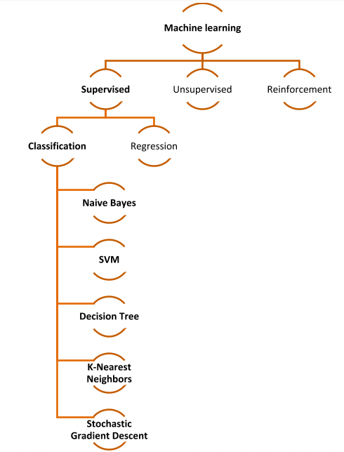
In classification, there are two types of learners –
- Lazy learners – These learners store the data and wait till the testing data is obtained. The most related data in the stored training data is used for classification resulting in more predicting time: for example, k-nearest neighbour.
- Early learners – These learn to train the model before receiving the testing data. The algorithm should come up with a general model that will work for all the datasets. For these learners, training time is more, but the prediction time is less. Example, Decision tree, Naïve Bayes.
How to Implement Classification In Machine Learning
Important terminologies in classification
- Classification model – a model is a generalised sequence of steps built using the training dataset and predicts the target class or category of new data
- Classifier – Algorithm that maps input data into a certain category
- Feature – property being observed in a dataset, for example, age, weight etc. are features
- Binary classification – classification type that has two possible outcomes – true/false, yes/no, 1/0
- multi-label classification – a type of classification where one data sample can be attached to multiple labels or categories
- multi-class classification – a classification that has more than two classes, but each sample can be attached to one label only
- Target prediction – The method or function that returns the output Y for input X using the function f(X) = Y
- Classifier training – Using the fit method to fit the model for training the input X and the label y.
- Evaluation – Checking for the accuracy and efficiency of the model built
Types of classification
There are four types of classification:
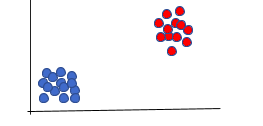
- Binary: These are classification tasks that have exactly two class labels. For example, whether a person is male or female, an email is spam or not, a person has a particular disease or not etc. Usually, these are represented by two states: normal (0) and abnormal (1). Some algorithms based on binary classification are logistic regression, Naïve Bayes, Decision tree, SVM. A binary classification task can be modelled using a model that predicts Bernoulli probability distribution, which covers cases where the output of an event is binary, i.e. 0 or 1. A scatter plot of binary classification will look like:
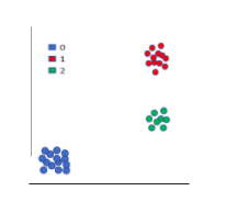
- Multi-class: These are classification tasks that have more than two class labels. For example, face classification (Google Photos), text/character recognition, flower classification etc. A multi-class classification task is modelled with a model that predicts a Multinoulli probability distribution, i.e. presence of a data point corresponding to each class label. Some popular algorithms used for multi-class classification are k-Nearest Neighbours, Decision Trees, Naive Bayes, Random Forest, Gradient Boosting.
You will notice that many binary classification algorithms are used for multi-class classifications as well as using one-vs-rest or one-vs-one fit. A scatter plot will be something like:
- Multi-label: In multi-label classification, each data point can have more than one class label. For example, object recognition. Suppose, there is an image, which has a horse, a cat and a dog. A second image might have a dog and a cat, and so on. If we see, the labels here are horse, cat, dog etc. This is different from multi-class where each data point will have only a label, i.e. each image will have only a horse OR cat OR dog but not more than one. Variations of the standard algorithms like decision trees, random forest and gradient boosting are used for multi-label classification.
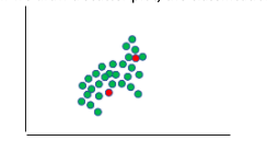
- Imbalanced: It is a special case of binary classification where there are more normal cases than abnormal cases. For example, Fraud detection, Outlier detection, Medical diagnostic tests. Specialised cost-sensitive versions of algorithms like Logistic Regression, Decision Trees, Support Vector Machines are used, and accuracy is measured using the metrics like Precision, Recall and F-measure.
If we draw a scatter plot, the classification will look like:
Important classification algorithms
There are many classification algorithms; some of the most popular ones are:
1. Logistic regression
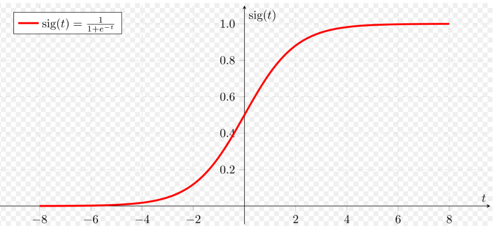
Logistic regression is the simplest algorithm and is used for binary classification of the data points. The categories are created such that each data point belongs to either of the two classes: 0 or 1. For example, whether we can play a cricket match today (yes/no). There are two parts to logistic regression: Hypothesis and Sigmoid Curve. Hypothesis determines the likelihood of an event and the data generated from the hypothesis fits into a log function creating an S-shaped curve called the ‘Sigmoid’. The category of the class can be predicted using the log function. The Sigmoid curve looks like an ‘S’:
Source: Wikimedia
As we see in the graph above, the function that represents this graph is the logistic function 1/(1+e-t), where e is the Euler’s number. The value of the curve always lies between 0 and 1. Hence, the equation for logistic regression is written as: y = e(b0 + b1*x) / (1 + e(b0 + b1*x)) Here, b0 and b1 are the two coefficients of the input x, estimated using the maximum likelihood estimation. Logistic regression is used in cases where we want to understand how a set of independent variables affect the output of the dependent variable. Logistic regression is simple but only works for binary outcomes and also assumes that the predictors are independent of each other, and the data doesn’t have any missing values. Some examples where logistic regression is used: word classification, disease detection, weather forecasting, voting applications.
2. Naïve Bayes
Naïve Bayes is particularly famous for its application in email spam detection. It is a powerful extension of the Bayes theorem. The ‘Naïve’ comes from the fact that the algorithm assumes that the features are independent of each other. It is quick and easy for predicting the class of a dataset and can be used for multi-class predictions. Naïve Bayes requires less training data. The fundamental principle behind the algorithm is the conditional probability (Bayes theorem), which states that, if X & Y are two independent variables, and the probability of occurrence of the event P(X|Y) is known. We can calculate P(Y|X) as: P(Y|X) = P(X|Y)*P(Y)/P(X) If the features X & Y are dependent, we would need huge data to determine P(X|Y) itself, which is impractical, thus the assumption that X & Y are independent. Note that the theorem can be extended to any number of features X as x1, x2, x3…. xn. Let us understand how Naïve Bayes performs spam filtering: consider that the spam messages are marked as ‘spam’ in the dataset. The other messages are marked as ‘ham’. We have to classify the data points to separate spam from ham. Example: spam: Winner!! Congratulations! You have won a cash prize of $200000. Claim it today! ham: Hey, it will be good to catch up on Thursday. Are you alright with it?
- The message is first to split into individual words.
- The data is then lemmatized (sorted into groups), same words with different tenses are considered to be one and replaced with the base word. For example, won, winner, winning, will be considered as win.
- Common words like a, is, the, it etc. are removed.
- Now, the spam detector algorithm (Naïve Bayes) is applied. In Python, the scikit-learn module is used (MultinomialNB).
- We can use the confusion matrix to determine the accuracy of the spam detector:
| Predicted class (P) | Predicted class (N) | |
| Actual class (P) | True Positive (TP) | False Negative (FN) |
| Actual class (N) | False Positive (FP) | True Negative (TN) |
Naïve Bayes makes a big assumption about the features being independent; however, in reality, there is some dependency between each input feature; hence they can be bad estimators in some cases. Although, when the assumption turns out to be right, they are fast, and require less amount of training data when compared to other algorithms. Naïve Bayes can also be used for sentiment analysis, document classification and disease prediction.
3. K-nearest neighbour
kNN is a lazy learning algorithm which is used for data mining, pattern recognition and intrusion detection. The algorithm doesn’t make any assumptions, unlike the other two algorithms we have seen earlier. kNN is a non-linear model that assigns data points to a cluster based on similarities. k is chosen randomly (usually 5). Then, take the sample you want to classify and find the k-nearest neighbours of the sample. Through majority vote, decide the class label for the sample. In the below case, we have three labels, , , . Now, if a new data point comes, we put it in the nearest cluster so that it can have a greater number of neighbours in that category.
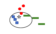
For example, We can see that the new data point, i.e. star, has five neighbours (k=5). A new point’s cluster is determined using its neighbours since this has three blue points, one green and one red, hence the new point (star) will be assigned to the blue cluster. k-NN works well even for large and noisy training data and is simple in implementation. However, the cost of computation is high compared to other algorithms. Some popular use cases of k-NN are in image recognition, handwriting detection, stock analysis, video recognition and other industrial applications.
4. SVM (including kernel trick)
SVM, aka Support Vector Machine, is used for classification as well as regression; however, classification is more common. The data points are first plotted in an n-dimensional space. Each feature represents a coordinate in the n-dimensional space. If there are two features, then we will have two coordinates, say X & Y. After plotting all the data points, an ideal hyperplane that differentiates the classes can be identified. The hyperplane should be close enough to both the classes and not just one class. As the number of features becomes more, the complexity of the algorithm becomes more. The steps to perform SVM are:
- Firstly, find the points that are closest to both the classes. These points are called support vectors.
- Next, we determine the proximity between the dividing plane and the support vectors.
- The distance between the points (SVs) and the dividing line is known as margin.
- SVM algorithm tries to maximize this margin, i.e. the optimal hyperplane is created when the margin reaches its maximum.
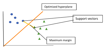
As we see above, SVM tries to maximize the distance between the two points (classes) by creating a well-defined boundary. We also see that the hyperplane is of 1-dimension and is a line. Therefore, in general, for an n-dimensional space, the hyperplane will be in (n-1) space, which will have disconnected components. SVM can be implemented easily in any language, be it Python, R or Matlab. It can be used for both linearly and nonlinearly separable data and also for labelled as well as unlabelled data. However, as we will see below, SVM uses kernel trick for feature mapping, which makes it difficult always to choose the right kernel. Tuning SVM parameters:
- Kernel: It transforms the input data into the desired format. Kernels can be radial, polynomial or linear depending on the number of features. It is important to choose the right kernel. Obviously, for non-linear hyperplane, radial and polynomial functions are used. SVM gives accurate classifiers with kernel transformation.
- Kernel trick: When we have too many features or a huge dataset, it is sometimes impossible to linearly separate the data. For this, we can project the data into a higher-dimensional space using a mapping function so that it becomes linearly separable. This hyperplane can then be used for classification. An example of kernel trick is as below:

Note that the first picture represents the data that is not linearly separable, after which we use the kernel trick (represented by the radial dashed circle). Then we look at the plane from a different view (think of looking at it from the right side). Then, you will be able to see a straight line, as shown in diagram 2.
- Regularisation: The next method to tune parameters is by adjusting the error value or the penalty parameter C, through which we can nullify the compensation between the decision boundary and the misclassified term. If C is small, the hyperplane will have a small margin, and if C has a larger value, the hyperplane will have a larger value.
SVM is used in many fields particularly for face detection, Bioinformatics, handwriting recognition, stock comparison, investment suggestions, document classification etc.
5. Decision tree
Decision trees are used for making decisions based on certain conditions or questions relevant to the features of the data and the main problem in hand. For example, if you want to decide whether you can eat an ice-cream for dinner, you should ask yourself: is it cold outside, do you have a cough or cold, is the shop open, is the flavour you want to have available and so on. If the answer to all these questions is favourable, then you can decide as ‘yes’ for the ice-cream. Here is a flowchart to visualize the same:
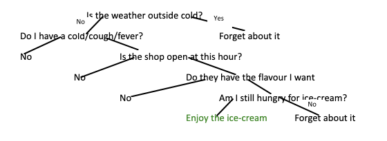
These are nothing but simple if-then rules which are mutually exclusive. The data is eventually broken down to smaller parts until the final termination point is reached. Decision trees require minimal data preparation and do not need any scaling. Also, we can fully understand the internal working of the model by visualising each step. Decision trees can handle categorical and numerical data. Some popular decision tree algorithms are:
- ID3 (Iterative Dichotomiser 3)
- C4.5 (successor of ID3)
- CART (Classification And Regression Tree)
- Chi-square automatic interaction detection (CHAID). Performs multi-level splits when computing classification trees.
- MARS: extends decision trees to handle numerical data better.
- Conditional Inference Trees: Statistics-based approach that uses non-parametric tests as splitting criteria corrected for multiple testing to avoid overfitting. This approach results in unbiased predictor selection and does not require pruning.
Check our detailed article on the implementation of Decision tree to know more about the working of this algorithm. Decision trees are very straightforward and simple, however very sensitive to data changes. Even a small data change can lead to changes in the whole tree structure, making the algorithm unstable. Some popular applications of the decision tree are pattern recognition, identifying disease severity and risks, data exploration, dynamic pricing, analysing customer satisfaction, sentiment analysis etc.
6. Random forest
A random forest is an ensemble of decision trees. They can be used for both classification and regression problems. Data is divided into subsets, and multitudes of decision trees are created during the training time. Training is done through bagging. The output is the mode or mean of the classes. Because of the presence of multiple decision trees, overfitting of the model is reduced, and the algorithm is more accurate than the decision tree itself. The accuracy keeps increasing as the number of trees increases. However, random forests are like black boxes and can’t be visualised, unlike decision trees. A random forest can be represented as:
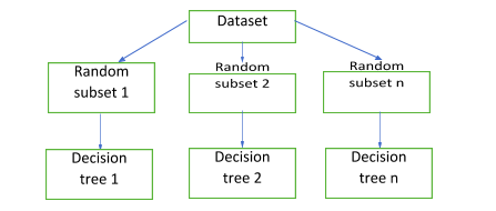
Let us understand the algorithm:
- The first step is to choose random samples from the training set. The number of samples n is ‘random’. This sample is called a bootstrap sample.
- From this sample, grow a decision tree and select d number of features at each node (randomly).
- Choose the feature that provides the best split amongst all the features. This is based on properties like information gain. The higher the value of information gain, the more important a particular feature is.
- If you want to create k numbers of trees, repeat the same process for all the k trees.
- Collate the prediction made by each tree and assign a new data point to the most popular group, i.e. group chosen by the maximum number of trees.
The most common applications of Random forest are in predicting social media share scores, finding loan eligibility and risk for an application, failure prediction, medical diagnosis, etc.
7. Artificial Neural networks
Neural networks try to mimic the human brain to make decisions. They consist of neurons that are arranged in various layers. There are three parts in an Artificial Neural Network (ANN): The input layer, hidden layer, output layer. There can be many hidden layers in a network, depending on the complexity of the problem. The workflow is usually a feed-forward one, i.e. from the input layer to the hidden layer and then to the output layer, with a feedback layer to the previous layer. Through the feedback, we can adjust the input weights and improve the accuracy of the NN. The algorithm to update the weights is called gradient descent. A simple neural network:
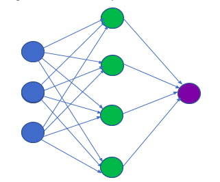
Here the blue circles indicate the inputs, green circles represent the hidden layers, and the output is the purple circle. This type of NN is called the feed-forward network, which has no feedback or back loops. Weights are applied to the inputs when they pass from layer to layer, and these weights are adjusted to tune the network during the training phase. In some neural networks, there is no hidden layer. Such networks have only two layers: input and output. These are called the perceptron. Perceptron takes input and adds weight to each input. Then, an activation function (for example, a sigmoid function) is applied to get the output for classification. Other types of neural networks are:
- Feed forward: These do not form a cycle and move only in the forward direction. All the nodes are fully connected. It is used for pattern recognition, speech recognition, computer vision, data compression etc.
- Radial Basis Network: These are popular for their application in function approximations and use Radial Basis function as the activation function. These are more suitable for continuous values and are used for time-series prediction, system control and classification.
- Deep Feed-forward: To reduce overfitting and improve generalisation, we can use more than one hidden layer. This is what Deep feed-forward networks do. It finds application in financial prediction, pattern recognition, data compression, ECG noise filtering, computer vision.
- Recurrent Neural network: If we want to access information from the previous layer in the current iteration itself, we use this type of NN. Each hidden layer receives the input with a specified time delay. Because of all this, the computational speed is low. RNN is one of the most popular NN and is used in Robot control, machine translation, time series prediction, speech recognition and synthesis, music composition and rhythm learning etc.
- Long/Short-Term Memory (LSTM): These networks have a memory cell to fetch very old data as well. LSTM is used for speech and writing recognition.
- Gated Recurrent Unit: This is a slight variation of LSTM, where-in there are three gates that do not maintain internal cell state: Update gate, Reset Gate, Current memory gate. These networks can be used for Polyphonic Music Modelling, Natural Language Processing, Speech Signal Modelling.
- Auto Encoder: Here, the number of hidden cells is smaller than the input cells. The output cells and input cells are the same. They are used in classification, regression and feature comparison.
There are many more popular NN, but the main working principle remains the same.
Implement Classification In Machine Learning - Key takeaways
To summarise the above section:
- We use classification algorithms to split data into categories called classes. The data can be linear or nonlinear.
- Naïve Bayes is the simplest classification algorithm that uses conditional probability to classify data
- Decision trees are powerful and can categorize data using splitting logic until no more splitting of nodes is needed
- Random forests are an extension of decision trees that perform more accurate predictions by ensemble learning
- Logistic regression classifies data based on sigmoid function and weighted parameters to determine the probability of the classes
- k-NN identifies closest neighbours or similarity in features to classify the data
- SVM creates the maximum margin hyperplane between the data classes to classify data
- Neural networks mimic the human brain and use ‘neurons’ to perform classification
How to select the right algorithm
There is no one way to select the right algorithm. If you have just started, you might have to try out multiple algorithms before you arrive at the most accurate and efficient one for a particular problem. The key is to create dependent and independent datasets based on features and divide the data into training and testing data. Sometimes, you may have to use more than one algorithm to train the model. That said, you can follow a pattern similar to this – if a dataset has less than 100k samples, use the SVC model, else go for SGD. If SGD doesn’t work, try kernel approximation, and if SVC doesn’t work, try k-NN. If that also doesn’t work, then go for Naïve Bayes or ensemble classifiers.
Checking the accuracy and efficiency
To check accuracy and efficiency, we need to evaluate the classifier. There are several methods to do the same:
- Holdout method: This is the most commonly used method for evaluating a classifier where data is split into train and test data. Mostly, data is split into the ratio 80:20 for train:test. The train dataset is used for training and building the model, where test data is used for evaluation.
- Cross-validation: Cross-validation is used to solve the problem of over-fitting in the model. An over-fitted model will not give the same accuracy for all the datasets because it is less generalized. K-fold cross-validation divides the dataset into k-subsets that are mutually exclusive, and one of the subsets is used for testing. The others are used for training the model. This process is repeated for all the k-folds.
- Classification report: The classification report gives the following:
-
- Accuracy: It is the ratio of correct observations (predicted) and the total observations. The number of correct positive predictions is called True Positive, and the number of correct negative predictions is called True negative.
- F1-Score: The weighted average of precision and recall
- Precision: Fraction of relevant instances amongst the retrieved instances
- Recall: Fraction of relevant instances retrieved over the total number of instances
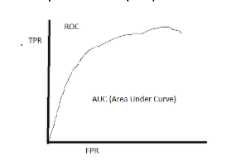
- <li">ROC Curve: ROC or Receiver Operating Characteristics performs a visual comparison of the classification models. It shows the relationship between the true positive rate (TPR) and the false positive rate (FPR). The area measures the accuracy of the model under the ROC curve.
Conclusion
In this article, we have discussed the various aspects of the most popular algorithms of classification. We have also discussed how to choose the right algorithm and test for accuracy. There are many more algorithms which are not covered in this article. To know more about machine learning , other types of algorithms and how to learn machine learning, check out the articles on our machine learning section . This is complete brief about How to Implement Classification In Machine Learning?
People are also reading:
- What is Machine Learning?
- Best Machine Learning Interview Questions
- Best Machine Learning Frameworks
- How to become a Machine Learning Engineer?
- Machine Learning Projects
- Classification in Machine Learning
- AI vs. ML vs. Deep Learning
- Machine Learning Applications
- Machine Learning Algorithm
- Data Science vs. Machine Learning
