
At each stage of the entire data science lifecycle, data scientists use various tools and techniques to get the best possible results. This blog discusses the various stages of the data science lifecycle and how datasets change after every stage. Data science is an interdisciplinary field that consists of many phases. Data scientists require many different skills like statistics, algebra, probability, programming, and domain knowledge to define business problems accurately and then solve them. Before diving into the data science lifecycle, we will first see the central component around which the entire data science is built – Data!
What is Data? – Lifecycle of Big Data
We are well aware that this is the age of big data. Because the traditional relational databases are no longer able to handle the amount of data generated per day, rather per second, the idea of big data came into the picture. Big Data refers to the process of storing and manipulating gargantuan amounts of - structured, semi-structured, and unstructured - data for data science purposes. Many big data frameworks , like Apache Hadoop, Spark, and Hive enable us to process data in a faster and more efficient manner. The lifecycle of data has become simple because of big data frameworks.
-
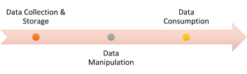
Data Disclosure
It involves the collection and storage of big data. To acquire or collect data, we use various data sources, including cloud, databases, and data warehouses, and pre-process the same to remove redundant, duplicate, or missing data. The resultant data is then stored appropriately using the big data storage systems, where data integrity and security are of the utmost importance.
-
Data Manipulation
After data disclosure, we aggregate and analyze the data. If there are multiple datasets, we combine them, and the ETL (Extract, Transform, and Load) process occurs. The resultant data is then analyzed, and reports are generated to take further action on the data.
-
Data Consumption
Once the final dataset is ready, it is ready to give maximum useful insights. One can use relevant data to generate information or knowledge or get business solutions that create more revenue or delete unwanted data.
Data lifecycle is a part of data mining, where data is acquired from various sources. Some analysis is performed on the data to make it usable for getting knowledge or insights.
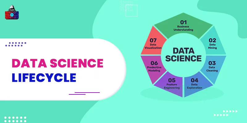
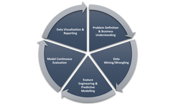
Data Science Lifecycle Stages
Now that we have seen how big data works, we will dive into the various stages of the data science lifecycle. Each stage is dependent on the next and also goes back to the previous stage if run into any errors. For example, if during Exploratory Data Analysis, we realized that all this while, we were using the wrong set of parameters, we would have to go back to the previous step, i.e., data acquisition, to get more relevant datasets. I have seen many blogs on the web, defining many stages that are confusing and similar. Here is a simple yet complete version that I have extracted based on my experience and some research from the web.
1. Problem Definition and Business Data Understanding
The first step of the data science lifecycle is to find out the business problem and give it a clear, actionable definition. To do this, you need to ask a lot of relevant questions and formulate hypotheses. If some supporting data is available, you should explore the data and arrive at some inference regarding defining the business problem. A hypothesis is nothing but an informed assumption about a particular target audience. Usually, a business problem is all about finding proof for the hypothesis. For example, if most 20-year-old girls prefer a specific hair color brand, a hypothesis can be made that it is the best brand out of all brands available in the market. To prove this hypothesis, however, we need more data like for how many days was this trend observed? Was the product offered at discount at that time? and so on. Suppose you are a competitor brand and this business problem is actual. Then the solution would be based on the data you collect and how you can improve sales of your brand by offering more unique hair colors, better price/discounts, perhaps a free service, et cetera. Excel is an excellent tool for writing down problem statements, and so are flowcharts and cause and effect matrices to define the problem.

2. Data Mining/Wrangling
Once we have defined our business problem, we need to find relevant data to support the hypothesis or find the solution to our problem. This step requires extensive research and data collection from various sources, like the internet, interviews, surveys, databases, legacy systems, cloud servers, and data warehouses. Multiple data sources are combined and integrated into a single large source through the mining process. Data mining is not just collecting data, instead, it involves pre-processing the data to find initial trends and patterns in the data to affirm that we are moving in the right direction in solving the business problem. If the insights we get through mining don’t support our initial statement, we have to go back to the first stage of (re)defining the business problem. Data mining is a big step and involves the following steps:
- Data collection through multiple sources.
- Understanding the data and how to make sense of it.
- Make it structured and usable by pre-processing, like aggregation, cleaning, and sorting.
- Transforming the data into a cleaner, better dataset.
- Exploratory Data Analysis (EDA) to find general trends and patterns.
Data sources can be offline resources, like journals, files, magazines, newspapers, interviews, questionnaires, and TV shows or online resources, like cloud servers, databases, and data warehouses. The pipeline, i.e., streaming or batch data, is another source of data for mining. Some
popular tools for data mining
are Knime, Weka, RapidMiner, Excel, and Spark.

3. Feature Engineering & Predictive Modeling
Once we have a clean dataset with some data analysis, we can decide the right parameters or features to help us create a model to solve our business problem. This means selection of most important features of data, determining dependent and independent variables, optimizing parameters, i.e., finding correlations between parameters, and reducing the total number of features using algorithms like Principal Component Analysis and Dimensionality Reduction. Once we have the features ready, we need to select an appropriate algorithm to train and test the model. We may need to apply more than one algorithm as algorithm and model selection are usually trial and error processes. Parameters should be tuned till we achieve a certain level of accuracy, and the model has to be continuously retrained based on feedback. Some popular feature engineering techniques are:
- Handling outliers,
- Binning,
- Imputation,
- Feature splitting,
- Log transform, and
- Scaling.
Some popular machine learning and deep learning algorithms for predictive modeling are:
- Classification models, like Naïve Bayes and SVM,
- Clustering models like k-means clustering,
- Regression models, like time-series and linear regression, and
- Neural networks.

4. Model Continuous Evaluation
Once the model is trained and deployed, it has to be thoroughly evaluated by using fresh (unknown) datasets. There are many methods to perform model evaluation, like model reporting, cross-validation, and A/B testing. Model evaluation should include all the aspects, like context evaluation, input evaluation, and performance evaluation, i.e., we have to see if the model can fit into the context and solve the purpose for which the model was built (called the goodness of fit). It should clearly define the dependent and independent variables and the relationship between them. Based on the performance of a model, it has to be either re-evaluated or accepted. Some statistical tools for model evaluation are:
-
Root Mean Square Error (RMSE)
RMSE is a reliable and robust metric for regression problems. When we take the root of all the numbers, the deviations appear larger. Similarly, taking squares of the numbers removes the negative error values, so the magnitude is always positive. If there are N observations, then RMSE is calculated as the sum of the squares of the difference between predicted and actual values, i.e.
RMSE = ?(?(predicted-actual)2)/N
-
Confidence Interval (CI)
CI is the amount of uncertainty in a sample of the dataset. The confidence level indicates the frequency of all the possible CIs that contain the ‘true’ value of the unknown parameter. Since it is an interval, CI is a range of values. If the population is more, the CI range will be less, thus giving more precise results.
-
Chi-square test
Used to test if there is any statistical difference between the observed value and the actual value, the Chi-square test is a hypothesis test. It is also known as the X2 test. It works on chi-squared distribution under the null hypothesis. First, we need to find the expected frequencies and the observed frequencies in the distribution. The sum (?) of the square of the difference between the expected frequency (fe) and observed frequency (fo) divided by the total expected frequency gives the chi-squared value:
X2 = (?(fo-fe)2)/fe
-
Confusion Matrix
A confusion matrix, represented by NxN, is also called an error matrix. We use a confusion matrix with classification models where N represents the number of classes (or categories) we want. We can see the true and false values in a visual representation using the confusion matrix as demonstrated below:
| Actual Class | Predicted Class | |||
| Positive | Negative | |||
| Positive | True Positive (TP) | False Negative (FN) ? Type II error | Sensitivity: TP/(TP+FN) | |
| Negative | False Positive (FP) ? Type I error | True Negative (TN) | Specificity: TN/(TN+FP) | |
| Precision: TP/(TP+FP) | Negative Predictive Value: TN/(TN+FN) | Accuracy: (TP+TN)/(TP+TN+FP+FN) | ||
-
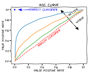
ROC (Receiver Operating Characteristic) Curve
ROC Curve is a graphical plot between the TPR (Sensitivity) and FPR (Specificity) at different threshold settings. FPR (False Positive Rate) is the probability of false alarm, i.e. (1-TPR) or one minus the True Positive Rate. It is generated by plotting the area under the probability distribution from minus infinity (-?) to the discrimination threshold.
 Source:
Wikipedia
Source:
Wikipedia
-
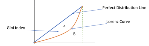
Gini Index
Gini Index is a statistical dispersion measurement. Used to calculate the purity of the decision tree, i.e., when a variable is randomly chosen as a feature, the Gini Index calculates the probability of the variable being wrongly classified so. The probability range is always between 0 and 1. To calculate Gini Index using a Lorenz-curve-based graph, we denote the same by A/A+B, where A and B are the areas represented as:
-
Cross-validation
Cross-validation is a statistical method to test the performance of a machine learning model on a new dataset. There are many methods to perform cross-validation like the hold-out method, k-fold cross-validation, and leave-p-out cross-validation.

5. Data Visualization and Business Reports
Many phases of the data science lifecycle leverage visualization. It is used to analyze all the relevant data in a single glance and understand quickly for further analysis and processing. It helps us to:
- Determine the important variables,
- Separate them from non-essential variables, and
- Find correlations between variables (columns of datasets).
Also, not all stakeholders and business analysts are technical people. To show them the outcomes of machine learning and the insights found by processing the data using all the above steps of the data science lifecycle, we need an interactive way that is also easily understood by everyone. This is possible through graphs and plots that present data in various ways. These are visualizations that can be easily explained, and all the insights can be seen at once. Data visualizations also consist of the business impact of the insights, the Key Performance Indicators (KPIs), the future plan to improve/solve the problem at hand. Some of the
popular visualization tools
are
Excel and Tableau
that provide different types of charts and visualizations suitable for various issues.

Conclusion
That sums up this article about the data science lifecycle. We saw that to solve a problem using data science, we require many steps. We collectively term these steps as the data science lifecycle. Each stage of the data science lifecycle is essential and makes the overall procedure much more comfortable and predictable. To further your data science knowledge, read what is Data Science? . You can further consider checking out the Data Science Roadmap to streamline your data science journey today! All the best. People are also reading:
- Data Scientist vs Data Analyst
- What is Data Engineering?
- Data Science vs Data Mining
- Python Data Visualization
- Artificial Intelligence Interview Questions
- Data Science Process
- Career Opportunities in Data Science
- Data Science Applications in Finance
- Top Data Science Skills
- Apriori Algorithm in Data Mining
- Python Data Science Libraries


Leave a Comment on this Post