
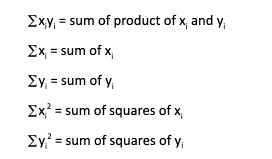
Statistics and probability are key to data analysis, manipulation, and formatting. Methods like mean, mode, median, standard deviation, etc., are used in almost all data science problems. In this article, we will discuss the most important and widely used methods of statistics and probability for data science.
Examples and Importance of Data
Data is a collection of information that you can collect from various sources. For example, details of a student or employee, like name, age, salary, marks, etc., are all essential data. In general, data can be factual or derived from other information. For instance, based on what a user orders on a food delivery app, we can analyze their taste and preferences. There are two types of data: Quantitative and Qualitative.
1. Quantitative data
It is countable, and it is to the point and conclusive. For example, if we have the average marks of two students as 89.7% and 84.3%, we can conclude that the former person is a better performer in academics.
Quantitative data is self-descriptive, and it is easy to plot a graph with quantitative data because it uses fixed values. It is possible to collect quantitative data through surveys, experiments, tests, market reports, metrics, etc. Quantitative data is further classified into two types, namely discrete and continuous.
- Continuous: Continuous values are the ones that you can break into smaller parts—for example, the speed of a train and the height, weight, and age of a person.
- Discrete: On the other hand, discrete values are integers that have a limit. For example, the number of people enrolled for a particular course, the cost of a new laptop, etc.
2. Qualitative data
It is unstructured (or semi-structured) and non-statistical. You cannot measure or plot such data using graphs. Such data can be classified using its attributes, labels, properties, and different identifiers. One typical example of qualitative data is the shopping preferences of a person.
Qualitative data often answers the question ‘why.’ This type of data helps to develop a hypothesis based on initial observations and understanding. The most common sources for collecting qualitative data are interviews, texts, documents, images, video transcripts, audio, and notes. Qualitative data is of two types, namely ordinal and nominal.
- Nominal: Nominal data is not in any particular order and is suitable for labeling. For example, the gender or hair color of a person.
- Ordinal: Ordinal data follow a particular order. For example, a survey form with answers categorized as good, very good, and excellent in order of preference.
Check out our article on Data Analysis Techniques to know the various techniques to analyze quantitative and qualitative data.
What is Statistics?
Statistics is the science of collecting vast amounts of numerical data for analysis, interpretation, and presentation of data for further use. It helps to obtain the right data, apply the best data analysis methods, and present the data in the most understandable and accurate form. Statistics is widely used in data science for analysis, interpretation, and presentation of data to make better decisions and predictions.
Jargons in Statistics
The most common terms used in statistics are as follows:
- Population: It is the entire pool of data or observations.
- Parameter: It is a numerical property of a population. For example, mean and median.
- Sample: A sample is a subset taken from a population.
- Statistic: A value that can be computed from the data that has known parameters.
- Random variable: Assignment of a number to all the possible outcomes of a random experiment.
- Range: Range is the difference between the largest and the smallest values in a set of data. For example, if the dataset has {1,2,3,4,5,6,7} as its values, the range is 7-1 = 6
- Mode: Mode is the most common value occurring in a list. Check out more statistics terms in this comprehensive glossary .
Types of Statistics
There are two types of statistics:
1. Descriptive statistics
Descriptive statistics are used to determine the basic features of data. You can get a summary of the sample and the measures. Every quantitative data analysis starts with descriptive statistics methods that define what the data contains. Also, it simplifies vast amounts of data through summaries like average, mean, etc. You can perform descriptive analysis in the following ways:
1.1 Univariate analysis
As the name says, it involves examining one variable at a time. We can look at the following characteristics of a single variable:
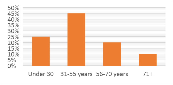
- Distribution: Distribution is the range of values for a variable, i.e., how the variable is distributed. For example, to represent the distribution of income among various age groups, we can divide them into different categories as per the range of values.
| Age | Percentage |
| Under 30 | 25% |
| 31-55 years | 45% |
| 56-70 years | 20% |
| 71+ | 10% |
The most common type of distribution (as shown above) is a frequency distribution. A frequency distribution can be represented graphically using a bar chart or histogram, as shown below:
1.2 Central Tendency
Central tendency is the measure of the central value in the range of data. The most common types of central tendency measures are – mean, median, and mode. Let us discuss them one by one.
Mean
It is the average value of all the values in the distribution. For example, the marks of a student in various subjects are 80, 82, 85, 89, and 93. Thus, the average or mean value will be the (sum of all the values/number of values) = (80 + 82 + 85 + 89 + 93)/5 = 85.8
Median
It is the value at the exact center of the entire distribution. For this, we have to sort the values in order: 80, 82, 85, 89, 93.
The middle value is = 85. Since we had five values, it was easy to find the middle. What if we had 6? Say, 80, 82, 85, 89, 93, 98. Now, the middle values are 85 and 89, and it's time to calculate the median. A common method to do this is to find the average. In this case, it will be (85+89)/2 = 87.
Mode
Mode is the most frequently occurring value in the distribution. Let us say there are a set of values {20, 25, 40, 40, 30, 20, 20, 35, 40, 45, 50, 30, 20}. We see that the value 20 occurs four times, which is the maximum among other values. So, the mode is 20. Sometimes, there might be more than one mode value in a given sample.
Dispersion
It is the spread of values around the central tendency. There are two ways to measure dispersion – range and standard deviation.
- Range: Range is the difference between the highest and the lowest value. For example, in {80, 82, 85, 89, 93}, the range is 93-80 = 13.
- Standard deviation: The problem with range is that if there is an outlier, the range value can change drastically. In the above example, what if the lowest value was 20 while all others in the distribution were above 80? That would radically change the range value. To avoid such a problem, we use the standard deviation.
Here's how you can calculate standard deviation:
Step 1 – First, calculate the mean (average) of the values. In our case, the mean is 85.8.
Step 2 – Calculate the distance of each value from the average value: 80 – 85.8 = -5.8 82 – 85.8 = -3.8 85 – 85.8 = -0.8 89 – 85.8 = +3.2 93 – 85.8 = +7.2
Step 3 – Square the differences -5.8 * -5.8 = 33.64 -3.8 * -3.8 = 14.44 -0.8 * -0.8 = 0.64 3.2 * 3.2 = 10.24 7.2 * 7.2 = 51.84
Step 4 – Calculate the sum of squares: 33.64 + 14.44 + 0.64 + 10.24 + 51.84 = 110.8
Step 5 – Divide this by the (number of values – 1). In our case, it is 4. 110.8/4 = 27.7. The above value is called the variance.
Step 6
– Calculate the standard deviation, which is the square root of the variance.
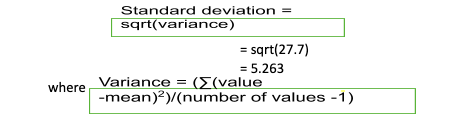
Standard deviation gives out a better spread of data or variation in data than range.
1.3 Correlation and Correlation matrix (Bivariate Analysis)
Correlation is one of the most widely used statistics for data science. It gives a single number as output that explains the degree of relationship between two variables. Here is an example to understand correlation: Consider a small dataset that contains details of the number of hours of activity and the happiness quotient of people.
Let us say we have a theory that more active people are happier. The activity can be of any type – exercising, pursuing a hobby like cooking, reading, etc. For simplicity, we will use the word ‘activity' for all the activities that require a person to be physically and mentally active.
| Person | Activity hours | Happiness quotient |
| 1 | 1 | 3 |
| 2 | 3 | 5 |
| 3 | 4 | 5 |
| 4 | 5.5 | 6 |
| 5 | 2 | 3 |
| 6 | 3 | 3.5 |
| 7 | 6 | 6 |
| 8 | 7.5 | 7 |
| 9 | 10 | 9 |
| 10 | 0 | 1 |
| 11 | 2.5 | 3 |
| 12 | 3.5 | 4 |
| 13 | 8.5 | 8 |
| 14 | 2 | 3.5 |
| 15 | 4 | 5.6 |
Let us first create a histogram for each and then find the other descriptive analysis parameters like mean, median, standard deviation, range, etc.
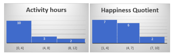 From the above, we can infer that the maximum number of people falls in the range of 0-4 hours of activity and a happiness quotient of 1-4.
How to Calculate Correlation?
Now, let us find some numerical data:
| Variable = Activity hours | Variable = Happiness Quotient | |
| Mean | 5 | 4.84 |
| Median | 3.5 | 5 |
| Variance | 7.988095238 | 4.605428571 |
| Standard Deviation | 2.826321857 | 2.146026228 |
| Range | 10 | 8 |
Note that these values can be easily calculated using Microsoft Excel. We can now plot a graph as well to determine whether the relationship between both the variables is positive or negative:
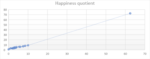
From the above graph, we can see that the relationship between the variables is positive, i.e., people who spend more hours doing various activities are happier. This proves the theory that we have discussed earlier with facts and data. The fact that the graph is moving in the upward direction indicates the same. This is precisely what correlation tells us.
Let us now calculate the correlation. Keep in mind that the formula for calculating correlation is a little complex, but all you have to do is remember just the formula, and there's no need to not how to derive it. Suppose x and y are the variables, and n is the number of items in the data. In our case, n = 15.
Now it's time to perform the calculation work (You can do most of it using Microsoft Excel). For our example, below are the calculated values:
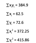
Now, let us apply all the values in the formula, r = (15*384.9-62.5*72.6)/?(15*372.25-62.52)*(15*415.86-72.62) = (5773.5-4537.5)/ ?(5583.75-3906.25)*(6237.9-5270.76) = (1236)/1273.726 r = 0.9704 Well, the correlation value for our data is 0.97, which is a perfect positive relationship between the two variables.
In general, the value of the coefficient is between -1.0 and +1.0, where the signs depict the negative and positive relationships, respectively. For the above example, we have calculated the Pearson Product Moment Correlation.
Correlation matrix
While we have taken an example that has two variables, real-world data will have many more variables. If we have to find the relationship between each of them, we will have to deal with several possible pairs. In general, the number of correlations is n(n-1)/2, where n is the number of variables. So, if we have five variables, we will have 5*4/2 = 10 correlations.
To represent all the correlations, we use a table: this table is called a correlation matrix. Below is what a correlation matrix looks like:
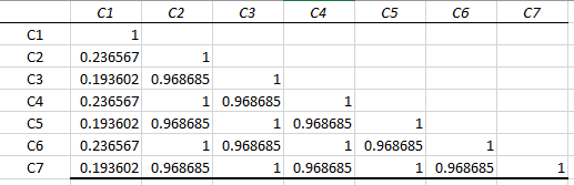
We can see that this is in the shape of a half triangle. The other half will be an exact mirror image of this, so we show only half a triangle of the matrix. A correlation matrix is always symmetric. So, let’s say you wanted to know the correlation value of C6 and C1; you just see C6 and the corresponding C1 value, i.e., 0.236567.
1.4 Entropy, information gain, and confusion matrix
Let us discuss each term separately to help you understand better.
Entropy
Entropy is the measure of impurity in a dataset. For example, if all the items in a group are of the same type, the impurity will be zero. If items are of a different kind, the impurity will be non-zero, i.e., the degree of randomness will be high when the items are of different types. Refer to our article on the decision tree in machine learning , to learn more about Entropy.
Information gain
Information gain measures how much information we can get from a particular variable or feature in the data. For example, if we want to identify how exercise affects a person’s health, and if the data contains a variable like ‘height,’ that variable will have low information gain as height is not a parameter to determine the effect of exercise on a person’s health.
Confusion matrix
The confusion matrix helps us examine the performance of a predictive model in classification problems. It is a tabular representation of the predicted vs. actual values to determine the accuracy of a model. Confusion matrix = (TP + TN)/(TP+TN+FP+FN) where TP = True Positive, TN = True Negative, FP = False Positive, and FN = False Negative A simple example to understand TP, TN, FP, FN is as follows:
Let us say we are given data about 20 students, of which 7 students are eligible for voter id, and 13 are not. We put this data into a model that predicts the outcome to be 8 eligible and 12 non-eligible students. With this, we can determine the accuracy of the model:
| number of samples = 20 | PREDICTED yes | PREDICTED no |
| ACTUAL yes | 7 (TP) | 1 (FN) |
| ACTUAL no | 2 (FP) | 10 (TN) |
TP represents the column where the actual and predicted both are yes, i.e., the actual and the predicted values both are yes. TN represents values where actual and predicted values both are no. FP indicates that something is not true (i.e., the students are not eligible), but the model predicted that it is true (i.e., the model predicted that they are eligible). FP is also called a type I error. FN indicates that something true is deemed as false by the model: The students are eligible, but the model predicted that they are not. FN is also called a Type II error.
2. Inferential statistics
In this type of statistical analysis, we try to extract information that that is evident from the data obtained, i.e., make inferences from the observations made through descriptive analysis. For example, if you want to compare the average marks obtained by students of two different colleges, you can use the t-test. There are many methods for performing inferential statistics, and most of them are based on the General Linear Model.
2.1 Paradigms for inference
There are several paradigms for inference that are not mutually exclusive. The four most common paradigms are as follows:
- Classical (frequentist) inference: Here, datasets similar to the one in question are said to be produced through the repeated sampling of population distribution. Examples – p-value and confidence interval.
- Bayesian inference: The Bayesian approach makes statistical propositions based on posterior beliefs. It is possible to describe degrees of belief using probability. Examples – interval estimation (credible interval) and model comparison using Bayes factors.
- Likelihood-based inference: This approach uses a likelihood function known as maximum likelihood estimation.
- AIC (Akaike Information Criterion) based inference: It is a measure of the relative quality of the statistical models, i.e., a pair (S, P), where S is the set of possible observations and P is the set of probability distributions for a given dataset.
2.2 Interval estimation
Interval estimation uses an interval or range of values to estimate a population parameter. The estimated value occurs between a lower and upper confidence limit. Let us say that you want to monitor your electricity bills. You get the bill amount to be somewhere between Rs.2000 and 3000. This is called an interval, where you don’t specify an exact value; instead, you specify a range or interval. Based on this, you can predict that the electricity bill for next month could also lie in the same interval. To statistically determine a population parameter, there are two essential terms we need to learn:
- Confidence interval: The measure of confidence that the interval estimate contains the population mean, i.e., uncertainty associated with a sample estimat3e
- Margin of error: It is the highest difference between the point estimate (the best estimate of a population parameter) and the actual value of the population parameter.
Maximum likelihood estimation
In this method, parameters of a probability distribution are estimated by maximizing a likelihood function by selecting parameter values that make the observed data the most probable. The point in the parameter space that maximizes the likelihood function is the ‘maximum likelihood estimate.’
How to perform inferential statistics?
There are several tests for inferential statistics. It is not a straightforward task to compute statistical inference, and the detailed calculations are beyond the scope of this article – each of the below methods needs a piece of its own for explanation and understanding. However, let's get a brief overview of these methods:
1. The t-test
The t-test or Turing test determines if the means of two groups are statistically different from each other. By this, we can know whether the probability of the results that we obtained are by chance or if they are repeatable for an entire population.
2. Dummy variables
It is a numerical value that represents the subgroups of the sample in consideration. A dummy variable is used in regression analysis and enables us to represent multiple groups using a single equation.
3. General Linear Model
GLM is the foundation for tests like the t-test, regression analysis, factor analysis, discriminant function analysis, etc. A linear model is generalized and thus useful in representing the relationship between variables through the following general equation: y = b0 + bx + e, where y is the set of outcome variables, x is the set of covariables, b is the set of coefficients (one for each x), and b0 is the set of intercept values.
4. Analysis of Covariance
ANCOVA is used to analyze the differences in the mean values of the dependent variables. These dependent variables are affected by controlled independent variables while taking into consideration the influence of uncontrolled independent variables. For example, how the eating patterns of customers will change if a restaurant is moved to a new location.
5. Regression-discontinuity analysis
The goal of this method is to find the effectiveness of a solution. For example, one person claims that following a proper diet plan can help reduce weight, a second person says that exercise is the most effective way to reduce weight, and another person believes that weight-loss pills help in faster weight loss. To find the outcome variable, we need to identify and assign participants that fit into each of these criteria (treatment groups).
6. Regression point displacement analysis
It is a simple quasi-experimental strategy for community-based research. The design is such that it enhances the single program unit situation with the performance of larger units of comparison. The comparison condition is modeled from a heterogeneous set of communities.
7. Hypothesis testing
In this inferential statistics technique, statisticians accept or reject a hypothesis based on whether there is enough evidence in the sample distribution to generalize the hypothesis for the entire population or not. This can lead to one of the following:
-
- Null hypothesis: The result is the same as that of the assumption.
- Alternate hypothesis : The result is different from the assumption made before.
An example of this can be a medicine for treating cough. If ten people take the medication daily, and they get relief from the cough on the 5th day, we can say that the probability that a person gets cured with the medicine in 5 days is high. However, if we take the data of 100 people and test the same on them, the results may vary. If those 100 also produce the same results, then we reach the null hypothesis. Else, if the majority of the 100 people do not get complete relief with the medicine in 5 days, then we reach an alternate hypothesis.
Sampling
The process of picking a certain part of data from the entire population for analysis is known as sampling. There are five types of sampling that are as follows:
- Random: In this type of sampling, all the members of the sample (or group) have equal chances of being selected.
- Systematic: In this type, every nth record from the population becomes a part of the sample. For example, out of numbers from 1-100 in a sample, we select the numbers at positions that are a multiple of 5, i.e., 5, 10, 15, etc.
- Convenience: This type of sampling involves taking samples from the part of the population that is closest or first to reach. It is also called grab sampling or availability sampling.
- Cluster: Samples are split into naturally occurring clusters. Each group should have heterogeneous members, and there should be homogeneity between groups. From these clusters, samples are selected using random sampling.
- Stratified: In this process, homogeneous subgroups are combined before sampling. Samples are then selected from the subgroups using random or systematic sampling methods.
What is Probability?
Probability is the measure of how likely it is for an event to occur. For example, if the weather is cloudy, the likelihood (or probability) of rain is high; if you roll a die, the probability of getting the number ‘6’ is 1/6; the probability of getting a ‘Queen’ from a pack of cards is 4/52. Similarly, the probability of getting a ‘queen of hearts’ from the pack is 1/52.
In general, you can calculate the probability of an event with the following formula:
Probability (event) = desired outcome/number of outcomes
Most problems in the real world do not have a definite yes or no solution, i.e., the likelihood or probability of the occurrence of an event can be more than another event. That’s why probability is so significant, and it is also one of the most critical topics of statistics.
Probability Jargons
- Event: The event is a combination of various outcomes. For example, if the weather is cloudy, there can be two possible events – rain or no rain.
- Experiment: It is a planned operation performed under controlled conditions. For example, getting Q of hearts on two successive picks from face cards is an experiment.
- Chance experiment: If the result of an experiment is not predetermined, such an experiment is called a chance experiment.
- Random experiment: It is an experiment or observation that can be repeated n number of times given the same set of conditions. The outcome of a random experiment is never certain.
- Outcome: The result of an experiment is called an outcome.
- Sample space: Sample space is the set of all the possible outcomes. Usually, the letter S is used to indicate sample space. If there are two outcomes of tossing a coin head (H) and tail (T), then the sample space can be represented as S = {H, T}.
- Likelihood: It is a measure of the extent to which the sample supports particular values of a parameter. Read more about likelihood vs. probability .
- Independent events: If the probability of the occurrence of an event doesn’t affect the probability of the other event in any way, such events are said to be independent events.
- Factor: A function that takes some number of random variables as an argument and produces output as a real number. Factors enable us to represent distributions in higher dimensional spaces.
Types of Probability
There are three main types of probabilities that form the foundation for machine learning. We have mentioned them below:
1. Marginal probability
Marginal probability indicates the probability of an event for one random variable amongst other random variables. Also, the outcome is independent of other random variables. P(A) = X for all outcomes of B The probability of occurrence of one event in the presence of a subset of or all outcomes from other random variables is called marginal distribution. In other words, the marginal probability distribution is the sum or union of all the probabilities of the second variable (B). P(A) = X or P(A=X) = sum (P (A=X, B=?Bi))
2. Conditional probability
It is the probability of the occurrence of an event A provided that another event B has occurred. The occurrence of event B is not certain, but it is not zero. A conditional probability distribution is the probability of one variable to one or more random variables. Conditional probability = P(A given B) = P(A|B) P(A given B) can be calculated with the following formula: P(A given B) = P(A and B)/P(B), where P(A and B) is the joint probability of A & B.
Bayes Theorem
Bayes's theorem is based on conditional probability. It describes the probability of event A based on the prior knowledge of conditions related to the event. The Bayesian theorem is also an approach for statistical inference or inferential analysis that we have discussed previously in this article and is key to Bayesian statistics . P(A|B) = P(B|A)*P(A)/P(B) where, P(A|B) = probability of A given B (conditional probability), P(A) & P(B) = probability of A & B respectively, P(B|A) = likelihood of B occurring given A is true
3. Joint probability
Joint probability is the probability of the occurrence of events A & B simultaneously and is represented as P(A and B). The joint probability of two or more events or random variables is called the joint probability distribution. It's easy to calculate joint probability; it is the product of the probability of event A given probability of event B and the probability of event B: P(A and B) = P(A U B) = P(A given B) * P(B) This calculation is also referred to as the product rule, and P(A given B) is the conditional probability. Remember that P(A U B) = P(B U A), i.e. joint probability is symmetrical.
Probability Distribution Functions
- Probability density function (Continuous probability distribution): It is a measure that specifies the probability of a random variable occurring between a specified range rather than a single value. The exact probability is found using the integral of the range of values of that variable. Moreover, when plotted on the graph, the graph looks like a bell curve, and the peak of the curve represents the model.
- Probability Mass function (Discrete probability distribution): It is a statistical measure to predict the possible outcome of a discrete random variable giving a single outcome value—for example, the price of stock or number of sales, etc. The values, when plotted on the graph, are shown as individual values, which should be non-negative.
- Normal (Gaussian) distribution : It is a type of continuous probability distribution and holds much importance in statistics. It allows the representation of real-valued random variables for which distributions are unknown. In a standard distribution curve, the data is centered around the curve, and the mean, mode, and median values are all the same. The graph is symmetrical about its center.
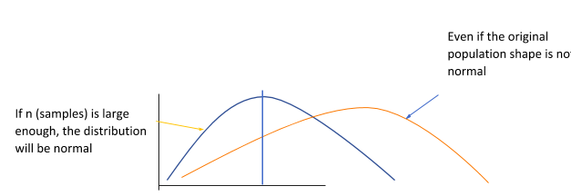
- Central limit theorem: This is a crucial concept in probability and statistics theory as it means that the methods of probability and statistics that work for normal distributions also work for many other types of distributions. CLT establishes that even if the original variables are not generally distributed after we add independent random variables, their properly normalized sum bends as a normal distribution curve. CLT comes in handy when the samples are high in number.
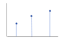
 Mean
Mean
Conclusion
We have discussed in detail the various statistics and probability methods used for data science. These are simple but vast and powerful. While doing data analysis, you need not remember the exact formulas. Instead, you can find them easily on the web; what’s important is to know when to apply which formula. The methods we discussed are just a small portion of the ways and algorithms used in data science. However, understanding these methods will create a strong base for your further exploration of the subject. It takes experience and time to grasp all the concepts of data science. However, you can easily achieve that with practice.
People are also reading:


Leave a Comment on this Post