

Python is the popular programming language for data science. As such, it has a galore of libraries and tools available that makes it easier to accomplish data science tasks. This blog details the best Python data science libraries. Data science, as you must be knowing, is a field that involves a lot of steps that help data scientists derive useful information from data and make business decisions. Typically, the entire data science lifecycle consists of the following steps:
- Collecting the data (Data collection) – surveys, crawlers, etc.
- Preparing the data (Data preparation) – cleaning, wrangling, processing, filtering, etc.
- Data mining – modeling, classification/clustering, etc.
- Analyzing the data (Data analysis) – exploratory, confirmatory, descriptive, predictive, regressive, qualitative analysis, etc.
- Data visualization – summarization, business intelligence, decision making, etc.
Each of these stages is a humongous process in itself, and if we were to do them manually, it would be an utter waste of resources and time. Instead, we can let the machines do most of this – through various libraries – so we can focus on the business aspects and reuse the code that's already there. Programming languages like Python offer a galore of packages to make data science tasks much more straightforward, which is why it is one of the most preferred languages for data science.
Stages of Data Science Lifecycle
You name the task, and Python gives a (or many) library to you. All you need to do is utilize it for your business scenario. Here are some essential libraries that you should know about if you are planning to tackle data science with Python:
- Data Collection: In this stage, data is collected from various sources. This could be from databases, clouds, interviews, surveys, etc. Some popular libraries used in this stage are Pandas, Beautiful Soup, and Requests.
- Data Preparation: Data preparation involves cleaning the raw data to make it suitable for further processing. This stage uses libraries like Pandas and Numpy.
- Data Processing: Data processing is the initial step of data analysis, where exploratory analysis is carried out to get the main features and statistical information about data. The main libraries used in this step are Pandas, Seaborn and matplotlib.
- Data Analysis: In this step, we train and build a model that helps us think about the best possible solution to the given problem. A problem can be in the form of classification or regression, and for each of these, there are many machine learning algorithms. Although it is difficult to determine which algorithm is the best for a particular problem, Python libraries like scikit-learn, TensorFlow and Gensim help identify the same, as many algorithms can be applied and results can be compared without much manual effort.
- Data Visualization: Presenting data is essential for making non-technical and business people understand what we want to convey. It also helps visualize the various approaches in a better way, making it easy to make decisions and form conclusions. Some popular libraries for visualization are seaborn, matplotlib, ggplot, and Plotly.
Best Python Data Science Libraries
In this section, let us dive deep into the Python data science libraries. This includes what the library contains and how it is useful in various stages of data science. We will also see how to install and import each of these libraries. So, here we go:
1. Pandas
As you would have noticed from above, Pandas is used in many stages of the data science lifecycle . It has compelling features like:
- Powerful data handling : Data handling capabilities through Dataframes and series. Through these, data can be represented and manipulated efficiently and quickly.
- Facilitates data manipulation: Indexing, organizing, labeling and alignment of data can be done using Pandas methods. This helps us view and manipulate data easily. For example, we can see just the first few items in a dataset with millions of records using Dataframe. One can create as many dataframes as needed and rename the columns to give them more recognizable labels. Without such methods, it will be impossible to view data and understand its main features.
- Handling missing data: Missing data can yield wrong results, and make the model inaccurate. Pandas handle missing data using the fillna() function, where missing values can be replaced by special values. Similarly, to check if a value is null, we can use functions like notnull() and isnull().
- Cleaning: Pandas have some great methods for data cleaning. For example, we can change the index of DataFrame and use the .str() method to clean columns. Same way, the .applymap() method can be used to clean the whole dataset, element-wise. Removing columns can be done simply by using the drop() method.
- Built-in functions for read and write operations: Pandas accepts many file types for reading and writing. There are various methods for writing and reading from different file types. For example, to write into .csv, we can use the to_csv() method of DataFrame and to read from CSV, we use the read_csv() method. The general syntax for methods is to_<filetype>() and read_<filetype().
- Combine Multiple Datasets: Usually, the complete data consists of data from various sources combined. It is difficult to manually merge data from various sources. However, Pandas makes it easy through various methods like:
-
- merge() – Joins data of common columns,
- join() – Combines data on one column, and
- append()/concat() – Combine dataframes across columns or rows.
- Visualization: Using Dataframe's plot() method, we can create various charts, and graphs like scatter plots, bar graphs, pie charts, and histograms.
- Statistical Functions: Methods like median(), mode(), std(), sum(), and mean() are commonly used for descriptive analysis. Further, the describe() function summarizes all the statistics at once.
How to Install and Import Pandas
If you have a Python Jupyter notebook, you can install and import Pandas right after installing Python itself. You can do so by using the code below:
pip install pandas
import pandas as pd
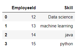
A simple example of a dataframe:
pd.DataFrame({"EmployeeId": [12, 13, 14, 15],
              "Skill": ['Data science', 'machine learning', 'java', 'python']})
2. Numpy
Numpy is one of the basic packages of Python, which helps you convert your data into n-dimensional arrays making data processing extremely useful and reduces the burden of scientific computations for developers. For example, here are the steps to create an array using Numpy:
pip install numpy
import numpy as np

arr = np.array( [[ 1, 2, 3], [ 4, 5, 6], [ 7, 8, 9]])
We can get the dimensions and type of array simply by using the methods arr.ndim and type(arr) , respectively. Numpy also offers methods for slicing, indexing and performing operations on arrays. For example, if we want to double the elements of an array arr = np.array([1, 2, 3]), we can simply use a = a*2, and the result will be [2, 4, 6]. Numpy also provides trigonometric functions like sin and cos. Same way, we can perform sorting of structured arrays by specifying the order. For example,
# define the data types for the array
dtypes = [('name', 'S10'), ('phone', int)]

# the actual array data
data = [('John', 7390898934), ('Mac', 8889283421),
           ('Joey', 8779233420), ('Dave', 8342287730)]

# create the array with data and data types
arr = np.array(data, dtype = dtypes)

# Sort the array with name
print ("\nSorted array by names:\n",
            np.sort(arr, order = 'name'))
Numpy can perform a lot more functions, and you can check them all on the official Numpy reference documentation page .
3. Seaborn
It is a visualization library built on matplotlib (that we will discuss next). Seaborn makes it easier to work with DataFrames as compared to matplotlib, but it is in no way a replacement for matplotlib. The Python data science library complements matplotlib beautifully and has many unique features like:
- Visualizing linear regression models,
- Styling graphics through built-in themes,
- Plotting time-series data, and
- Viewing bivariate and univariate data.
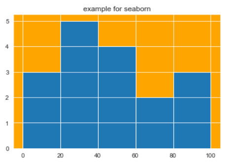
You will still need to import and use matplotlib to plot the basic graph and then set styles and scales using seaborn. There are 5 themes available in the latest version of Seaborn – dark, white, ticks, darkgrid, and whitegrid. Among these, darkgrid is the default style. To remove the right and top axes, we can use the despine() function (which is not available in matplotlib). A lot of customizations are possible using the set_styles() method, to which you can pass parameters like font.family, axes.grid, grid.color, xtick.color, ytick,direction, and figure.facecolor. We can enhance the aesthetics of plots by giving various colors using the color_palette() function. Here is a simple histogram using Seaborn. To install Seaborn, use pip install seaborn. Below is an example of using Seaborn:
import numpy as np
from matplotlib import pyplot as plt
import seaborn as sb

sb.set_style("darkgrid", {'axes.axisbelow': False, 'axes.facecolor': 'Orange'})

a = np.array([12,88,45,47,80,73,43,84,12,20,34,45,79,26,37,39,11])
plt.hist(a, bins = [0,20,40,60,80,100])
plt.title("example for seaborn")
plt.show()
This will give the output as:
4. Matplotlib
We have already seen how simple it is to use matplotlib in the previous section. It is the main library for data visualization and contains loads of methods to plot any type of graphs and charts. Some important features of matplotlib are:
- Most suitable and commonly used library for 2D plots.
- Any type of plot can be created using this library like the bar, line, scatter, and pie.
- Multiple subplots can be easily created using the subplot() function.
- Matplotlib can also display images using the imshow() function.
- Also supports 3D graphs like surface, scatter, and wireframe.
- Supports streamplots and ellipses.
- The name comes from its MATLAB-like interface ('mat" plot" lib') for plots.
How to Install and Import matplotlib
These are the installation and import statements for matplotlib:
pip install matplotlib
from matplotlib import pyplot as plt
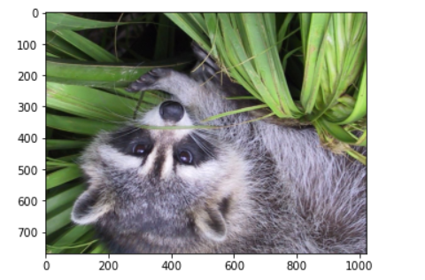
#get face image of panda from misc package
panda = misc.face()
# rotate it for some fun; you can skip this if you don't want to rotate your image
panda_rotate = ndimage.rotate(panda, 180)
plt.imshow( panda_rotate)
plt.show()
matplotlib Examples
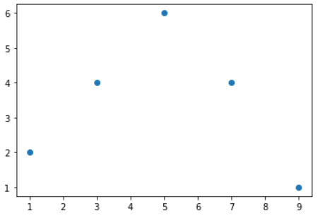
A simple scatter plot using matplotlib:
from matplotlib import pyplot as plt
# x-axis values
x = [1, 3, 5, 7, 9]
# Y-axis values
y = [2, 4, 6, 4, 1]
# Function to plot scatter
plt.scatter(x, y)
# function to show the plot
plt.show()
Here is a simple 3D plot using matplotlib. Note that to plot 3D graphs, we need the mpl_toolkits package. It is automatically installed when you install the matplotlib package:
from mpl_toolkits import mplot3d
import numpy as np
import matplotlib.pyplot as plt
fig = plt.figure()

def func(x, y):
    return np.cos(np.sqrt(x ** 2 + y ** 2))
# create evenly spaced sequences of the given intervals
x = np.linspace(-5, 5, 20)
y = np.linspace(-5, 5, 20)

X, Y = np.meshgrid(x, y)
Z = func(X, Y)
fig = plt.figure()
#this will create a 3d mesh grid
ax = plt.axes(projection='3d')
# You can use the method contour3D as well (try it!)
ax.contourf(X, Y, Z)
ax.set_xlabel('x')
ax.set_ylabel('y')
ax.set_zlabel('z');
#to view at a different angle, use the property view_init
ax.view_init(45, 30)
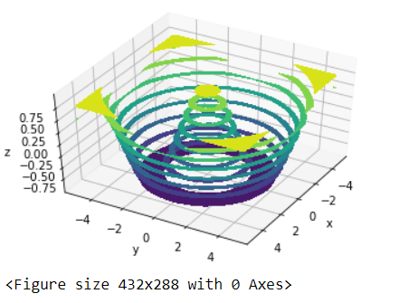
In this section, we have seen some advanced functions of both matplotlib and Numpy. Notice that many Python data science libraries work together to produce the desired results.
5. Scikit-learn
A must-have library for machine learning, this package contains all the ML algorithms you can think of. From classification to regression, dimensionality reduction to clustering, you will find all of them. Scikit-learn is built on top of other Python data science libraries, like scipy, NumPy and matplotlib. You can reuse the code in various contexts. Scikit-learn also provides methods to split the data into training and testing sets, and test the accuracy of the model in case of a supervised learning model. You can also use more metrics to use the newly added cross-validation feature. The package comes with sample datasets that you can use for practice, for example, the iris dataset. To access the features of the dataset, you can use .data member.
How to Install and Import Scikit-learn
from sklearn import datasets
iris = datasets.load_iris()
print(iris.data)
For the sake of simplicity in understanding, let us take this dataset itself to explore the various models of scikit-learn. Let us say we want to predict the probability of a particular iris to be of type setosa. We will start with the simplest of all algorithms – the Naïve Bayes. Look out for the explanation of the code in the inline comments:
from sklearn import datasets
import pandas as pd
from sklearn.naive_bayes import GaussianNB
iris = datasets.load_iris()
#set the petal width
X = iris["data"][:,3:]
# our target type is setosa, whose int value as we gather from the dataset is 0
y = (iris["target"]==0).astype(np.int)

#We use the gaussian formula for classifier
clf = GaussianNB()
clf.fit(X,y)
X_new = np.linspace(0,6,100).reshape(-1,1)

# predict the probability of the new data being setosa

y_proba = clf.predict_proba(X_new)

# Plot the data
plt.plot(X,y,"b.")
#find the probability; remember our target is setosa
plt.plot(X_new,y_proba[:,1],"r",label="Iris-Setosa")
plt.plot(X_new,y_proba[:,0],"b",label="Not Iris-Setosa")
# these are for the text to appear
plt.xlabel("Petal width", fontsize=10)
plt.ylabel("Probability", fontsize=10)
plt.legend(loc="upper right", fontsize=10)
plt.show()
When we plot the data, we get the probability value between 0 and 1 as:
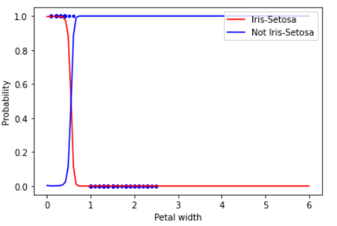
sklearn has classes for each algorithm. For example, for logistic regression, you will import the same from a linear model:
from sklearn.linear_model import LogisticRegression
For Random forest, you will use,
from sklearn.ensemble import RandomForestClassifier
Use from sklearn.cluster import KMeans for the K-means algorithm, and so on. sklearn has a function train_test_split that makes partition in data for training and testing purposes.
6. Requests
As the name suggests, Requests is a module that handles all types of HTTP requests. It is easy to use and has many features, like adding headers, passing URL parameters, and SSL verification. You can use pip install requests to install Requests. When we use the GET method, we get a detailed response too:
import requests
resp = requests.get('https://www.techgeekbuzz.com/')
We can print individual elements of the response using the code below:
print(resp.encoding)
print(resp.status_code)
print(resp.elapsed)
print(resp.url)
print(resp.headers['Content-Type'])
We can send a query string as a dictionary containing strings using the params keyword. For example:
query = {'s': 'supervised+learning'}
resp = requests.get('https://www.techgeekbuzz.com/', params=query)
print(resp.url)
Similarly, we can use the POST method too. Post methods are useful for submitting forms automatically. An example of the same is:
resp = requests.post('https://www.techgeekbuzz.com', data = {'search':'Data Science'})
resp.raise_for_status()
with open('what-is-data-science', 'wb') as filed:
    for chunk in resp.iter_content(chunk_size=100):
        filed.write(chunk)
print(filed)
The above code will write the contents of the page 'what-is-data-science' into a file for up to the size 100. We have set it to 100 for the sake of simplicity. You can increase the number to 50,000 or more. Requests also allows you to set cookies, session objects, and headers. The Python data science package is helpful when you want to scrape webpage information from the web.
7. PyTorch and TensorFlow
PyTorch is an open-source library, explicitly used for applications like Natural Language Processing and computer vision. It provides tensor computing through Graphics Processing Unit (GPU) and deep neural networks. It defines Torch.tensor class to work on homogeneous rectangular arrays of numbers. Companies like NVIDIA and AMD use PyTorch. We have already explored how Numpy can do scientific computations. However, it is slow and cannot utilize GPUs for faster computations. The fundamental concept of PyTorch, i.e. a Tensor is also an n-dimensional array, but along with scientific computations, it can also take care of gradients and computational graphs. PyTorch has many methods to manipulate Tensors.
But what is a tensor?
As we mentioned before, a Tensor is an n-dimensional array, rather than a vector or matrix that can represent any type of data. A tensor holds values of the same data type with a known shape. The shape of the data represents the dimensionality of the matrix/array/vector. Data scientists widely use PyTorch. The Python data science library is also used by AI developers, researchers and machine learning experts for deep learning models. It is flexible, has a simple interface, and offers dynamic computational graphs.
So, why, TensorFlow?
PyTorch is more intuitive than TensorFlow. You can create graphs on the go with PyTorch, whereas TensorFlow can create only a static graph, i.e. before you run the model, you should have defined the entire computational graph. It is also much easier to learn than TensorFlow. As you might have guessed by now, TensorFlow is a library, similar to PyTorch, used for deep learning. TensorFlow, developed by Google, is based on Theano while PyTorch, developed by Facebook, is based on the now-defunct Torch. TensorFlow is relatively more established and has a bigger community, more tutorials and resources for learning. For production-ready scalable projects, TensorFlow is more suitable. It also has a visualization tool, Tensorboard, through which you can view ML models in the browser itself.
How to Install TensorFlow
To install TensorFlow, you need to install Anaconda and then create a .yml file to install the dependencies. Then use pip install tensorflow to add Tensorflow. Now, open the .yml file and add the following code:
name: <filename>
dependencies:
- python=3.6
- jupyter
- ipython
- pandas
The above code, when run, will install the dependencies mentioned. Compile the .yml file using conda env create -f <filename>.yml command and activate the file using the active <filename> command. After installation, check whether all the dependencies are installed and then install TensorFlow using the pip command mentioned above. The next step is to import and use it! This is how to do it:
import tensorflow as tf
hi = tf.constant("Hey there, good evening!")
hi
TensorFlow conducts all operations in a graph, i.e. computations take place successively. The nodes are connected, and each operation is called an op node. The main input to a tensor is the feature vector, which then goes through an operation and creates a new tensor which is fed to another operation. Since tensors work on 3 or more dimensions, they have 3 properties:
- label (name),
- data type and
- a shape or dimension.
For example:
        tens1  = tf.constant(12, tf.int16) will produce output as,
Tensor("Const:0”, shape=(), dtype=int16)
In the order name, shape and data type, respectively. Data type can be anything from float32, string, bool, etc. If a function is applied to the value:
       X = tf.constant([3.0], dtype = tf.float32)
   print(tf.sqrt(X))
The tensor object will now have a shape value:
Tensor("Sqrt:0", shape=(1,), dtype=float32)
This is just to show you the basics of TensorFlow objects. The detailed explanation of TensorFlow is beyond the scope of this article and will be covered separately in another article. You can learn more about TensorFlow from the official website .
8. Arrow
Arrow is specifically to handle date, time and timestamp. Usually, date and time become a big headache to work with and need extensive coding. With Arrow, this constraint can be removed. Arrow has a lot of features like:
- Very simple creation options for standard inputs.
- Time Zone conversions; UTC by default.
- Generates ranges, floor, ceiling, time span for time frames from microseconds to years.
- Supports locales.
- Support for relative offsets.
- Extensible.
You can install Arrow using pip install Arrow and then import it using import arrow statement. A simple example:
import arrow as ar
utc = ar.utcnow()
utc
<Arrow [2020-07-22T18:38:12.126947+00:00]>

local = utc.to('UTC-5')
local
<Arrow [2020-07-22T13:44:32.675160-05:00]>
Arrow can search a date in a string and parse it, for example:
ar.get('I was born on 05 September 1975', 'DD MMMM YYYY')
<Arrow [1975-09-05T00:00:00+00:00]>
You can humanize the time, such as:
now = ar.utcnow()
later = now.shift(hours=4)
later
This will give output as <Arrow [2020-07-22T22:53:55.509976+00:00]> If you humanize:
later.humanize(now),
You will get:
'in 4 hours'
The API is self-explanatory, and functions are exhaustive yet simple to understand. You can use Arrow whenever your project requires extensive date manipulation and working with date ranges.
9. Beautiful Soup
Beautiful soup scrapes information from websites for mining. It is written in an HTML file or XML parser and creates a parse tree that gathers data from HTML. The installation process is the same as for other Python data science libraries:
pip install beautifulsoup4
from bs4 import BeautifulSoup

soup = BeautifulSoup('https://www.techgeekbuzz.com', 'html.parser')
Once you create a soup object, you can use methods like findall() , prettify() , and contents to extract data from the HTML files.
How to Create a Custom Library in Python?
So, that was about some of the most popular and widely used Python data science libraries. Now, let's talk a little about creating your own library in Python. Python is one of the most popular languages for data science, mainly because of the built-in libraries it supports. However, if as a developer you still feel that there is something for which a library has not yet been developed, and you can reuse the code for other purposes too, Python allows you to create custom libraries too. A Python library is nothing but a collection of Python modules that are organized in a package. It is very simple to create a module. This is how to do so:
def myownfunc(param):
print(param)
After creating the module, save the file with an appropriate name (say, myownmodule) and a .py extension.
To use this module, use the following code:
import myownmodule
myownmodule.myownfunc(a)
The next step is to package this module into a library. We can add more modules and combine all of them into one library. We do this using the setup module. First, create setup.py in the root directory of the package and then run python setup.py sdist_distrname to create the source distribution. Running the aforementioned code will create a tar-gzipped file, stored under the dist (distribution) directory. For others to use this package, you have to upload it to PyPI (Python Packages Index). This requires registration and the creation of a new account on PyPI. You can then upload your package using twine.
Why Python Data Science Libraries?
We have already explored the use of various Python data science libraries in the article. If we have a library, we can reuse the code already written by somebody else for the same purpose. This saves a lot of time and resources and helps businesses focus on their business logic alone. Further, in Python, it is easy to find out which library can be used for what purpose by using the 'help' option. We can also create custom libraries and modules in Python that, when distributed can be used by others. Doing so, thus, helps in building a strong community and network of developers.
Conclusion
"How is a package different from a library?" Is this on your mind? The main difference is that functions and modules in a library may or may not be related to each other but are put together as one so that you can build your program over it. The programs in a package, on the contrary, are closely related to each other. A library consists of many packages that serve different purposes. The above list of Python data science libraries is in no way comprehensive. There are many libraries like Keras, ggplot, Plotly, and Scraper that are very useful too. The libraries you choose depend on your business needs and use-cases, but the basic ones like Numpy, Pandas, Matplotlib and scikit-learn are used in almost all data science and machine learning problems.
Let us know in the comments if you want us to write about a specific Python library!
People are also reading:
- Extract Image Metadata in Python
- How to Read Emails in Python?
- Crack PDF Files Passwords in Python
- Python Make a URL Shortner
- How to Get Geolocation in Python?
- Python SIFT Feature
- Python Extract Images from PDF
- Extract all PDF Links in Python
- SYN Flooding Attack in Python
- Extract YouTube Comments in Python


Leave a Comment on this Post